Casual Inference Data analysis and other apocrypha
Describing and Forecasting time series: Autoregressive models in Python

Plenty of problems confronted by practicing data scientists have a time series component. Luckily, building time series models for forecasting and description is easy in statsmodels. We’ll walk through a forecasting problem using an autoregressive model with covariates (AR-X) model in Python.
Time series data is everywhere
For practicing data scientists, time series data is everywhere - almost anything we care to observe can be observed over time. Some use cases that have shown up frequently in my work are:
- Monitoring metrics and KPIs: We use KPIs to understand some aspect of the business as it changes over time. We often want to model changes in KPIs to see what affects them, or construct a forecast for them into the near future.
- Capacity planning: Many businesses have seasonal changes in their demand or supply. Understanding these trends helps us make sure we have enough production, bandwidth, sales staff, etc as conditions change.
- Understanding the rollout of a new treatment or policy: As a new policy takes effect, what results do we see? How do our measurements compare with what we expected? By comparing post-treatment observations to a forecast, or including treatment indicators in the model, we can get an understanding of this.
Each of these use cases is a combination of description (understanding the structure of the series as we observe it) and forecasting (predicting how the series will look in the future). We can perform both of these tasks using the implementation of Autoregressive models in Python found in statsmodels.
Example: Airline passenger forecasting and the AR-X(p) model
We’ll use a time series of monthly airline passenger counts from 1949 to 1960 in this example. An airline or shipping company might use this for capacity planning.
We’ll read in the data using pandas:
import pandas as pd
from matplotlib import pyplot as plt
import numpy as np
from patsy import dmatrix, build_design_matrices

df = pd.read_csv('airline.csv')

df['log_passengers'] = np.log(df.Passengers)

df['year'] = df['Month'].apply(lambda x: int(x.split('-')[0]))
df['month_number'] = df['Month'].apply(lambda x: int(x.split('-')[1]))
df['t'] = df.index.values
Then, we’ll split it into three segments: training, model selection, and forecasting. We’ll select the complexity of the model using the model selection set as a holdout, and then attempt to forecast into the future on the forecasting set. Note that this is time series data, so we need to split the data set into three sequential groups, rather than splitting it randomly. We’ll use a model selection/forecasting set of about 24 months each, a plausible period of time for an airline to forecast demand.
Note that we’ll use patsy’s dmatrix to turn the month number into a set of categorical dummy variables. This corresponds to the R-style formula C(month_number)-1; we could insert whatever R-style formula we like here to generate the design matrix for the additional factor matrix $X$ in the model above.
train_cutoff = 96
validate_cutoff = 120

train_df = df[df['t'] <= train_cutoff]
select_df = df[(df['t'] > train_cutoff) & (df['t'] <= validate_cutoff)]
forecast_df = df[df['t'] > validate_cutoff]

dm = dmatrix('C(month_number)-1', df)
train_exog = build_design_matrices([dm.design_info], train_df, return_type='dataframe')[0]
select_exog = build_design_matrices([dm.design_info], select_df, return_type='dataframe')[0]
forecast_exog = build_design_matrices([dm.design_info], forecast_df, return_type='dataframe')[0]
Let’s visualize the training and model selection data:
plt.plot(train_df.t, train_df.Passengers, label='Training data')
plt.plot(select_df.t, select_df.Passengers, label='Model selection holdout')
plt.legend()
plt.title('Airline passengers by month')
plt.ylabel('Total passengers')
plt.xlabel('Month')
plt.show()
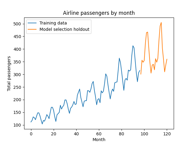
We can observe a few features of this data set which will show up in our model:
- On the first date observed, the value is non-zero
- There is a positive trend
- There are regular cycles of 12 months
- The next point is close to the last point
Our model will include:
- An intercept term, representing the value at t = 0
- A linear trend term
- A set of lag terms, encoding how the next observation depends on those just before it
- A set of “additional factors”, which in our case will be dummy variables for the months of the year
- A white noise term, the time-series analogue of IID Gaussian noise (the two are not quite identical, but the differences aren’t relevant here)
Formally, the model we’ll use looks like this:
\[log \underbrace{y_t}_\textrm{Outcome at time t} \sim \underbrace{\alpha}_\textrm{Intercept} + \underbrace{\gamma t}_\textrm{Trend} + \underbrace{(\sum_{i=1}^{p} \phi_i y_{t-i})}_\textrm{Lag terms} + \underbrace{\beta X_t}_\textrm{Extra factors} + \underbrace{\epsilon_t}_\textrm{White Noise}\]The model above is a type of autoregressive model (so named because the target variable is regressed on lagged versions of itself). More precisely, this gives us the AR-X(p) model, an AR(p) model with extra inputs.
As we’ve previously discussed in this post, it makes sense to take the log of the dependent variable here.
There’s one hyperparameter in this model - the number of lag terms to include, called $p$. For now we’ll set $p=5$, but we’ll tune this later with cross validation. Let’s fit the model, and see how the in-sample fit looks for our training set:
from statsmodels.tsa.ar_model import AutoReg

ar_model = AutoReg(endog=train_df.log_passengers, exog=train_exog, lags=5, trend='ct')
ar_fit = ar_model.fit()

train_log_pred = ar_fit.predict(start=train_df.t.min(), end=train_df.t.max(), exog=train_exog)

plt.plot(train_df.t, train_df.Passengers, label='Training data')
plt.plot(train_df.t,
         np.exp(train_log_pred), linestyle='dashed', label='In-sample prediction')
plt.legend()
plt.title('Airline passengers by month')
plt.ylabel('Total passengers')
plt.xlabel('Month')
plt.show()
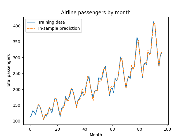
So far, so good! Since we’re wary of overfitting, we’ll check the out-of-sample fit in the next section. Before we do, I want to point out that we can call summary() on the AR model to see the usual regression output:
print(ar_fit.summary())
                            AutoReg Model Results
==============================================================================
Dep. Variable:         log_passengers   No. Observations:                  121
Model:                  AutoReg-X(17)   Log Likelihood                 224.797
Method:               Conditional MLE   S.D. of innovations              0.028
Date:                Fri, 16 Jul 2021   AIC                             -6.546
Time:                        10:11:20   BIC                             -5.732
Sample:                            17   HQIC                            -6.216
                                  121
=======================================================================================
                          coef    std err          z      P>|z|      [0.025      0.975]
---------------------------------------------------------------------------------------
intercept               1.0672      0.461      2.314      0.021       0.163       1.971
trend                   0.0023      0.001      1.980      0.048    2.31e-05       0.005
log_passengers.L1       0.6367      0.092      6.958      0.000       0.457       0.816
log_passengers.L2       0.2344      0.109      2.151      0.031       0.021       0.448
log_passengers.L3      -0.0890      0.111     -0.799      0.425      -0.308       0.129
log_passengers.L4      -0.1726      0.110     -1.576      0.115      -0.387       0.042
log_passengers.L5       0.2048      0.108      1.900      0.057      -0.007       0.416
log_passengers.L6       0.0557      0.111      0.504      0.615      -0.161       0.272
log_passengers.L7      -0.1228      0.110     -1.113      0.266      -0.339       0.093
log_passengers.L8      -0.0741      0.111     -0.667      0.505      -0.292       0.143
log_passengers.L9       0.1571      0.111      1.418      0.156      -0.060       0.374
log_passengers.L10     -0.0411      0.112     -0.367      0.713      -0.260       0.178
log_passengers.L11      0.0325      0.111      0.292      0.771      -0.186       0.251
log_passengers.L12      0.0735      0.112      0.654      0.513      -0.147       0.294
log_passengers.L13      0.0475      0.111      0.429      0.668      -0.169       0.264
log_passengers.L14     -0.0263      0.109     -0.240      0.810      -0.241       0.188
log_passengers.L15      0.0049      0.109      0.045      0.964      -0.208       0.218
log_passengers.L16     -0.2845      0.105     -2.705      0.007      -0.491      -0.078
log_passengers.L17      0.1254      0.094      1.339      0.181      -0.058       0.309
C(month_number)[1]      0.0929      0.053      1.738      0.082      -0.012       0.198
C(month_number)[2]      0.0067      0.050      0.134      0.893      -0.091       0.105
C(month_number)[3]      0.1438      0.044      3.250      0.001       0.057       0.230
C(month_number)[4]      0.1006      0.045      2.233      0.026       0.012       0.189
C(month_number)[5]      0.0541      0.048      1.123      0.261      -0.040       0.149
C(month_number)[6]      0.1553      0.047      3.290      0.001       0.063       0.248
C(month_number)[7]      0.2453      0.050      4.897      0.000       0.147       0.343
C(month_number)[8]      0.1108      0.056      1.990      0.047       0.002       0.220
C(month_number)[9]     -0.0431      0.055     -0.785      0.433      -0.151       0.065
C(month_number)[10]     0.0151      0.053      0.283      0.777      -0.089       0.120
C(month_number)[11]     0.0165      0.053      0.311      0.756      -0.087       0.120
C(month_number)[12]     0.1692      0.053      3.207      0.001       0.066       0.273
In this case, we see that there’s a positive intercept, a positive trend, and a spike in travel over the summary (months 6, 7, 8) and the winter holidays (month 12).
Model checking and model selection
Since our in-sample fit looked good, let’s see how the $p=5$ model performs out-of-sample.
select_log_pred = ar_fit.predict(start=select_df.t.min(), end=select_df.t.max(), exog_oos=select_exog)

plt.plot(train_df.t, train_df.Passengers, label='Training data')
plt.plot(select_df.t, select_df.Passengers, label='Model selection holdout')
plt.plot(train_df.t,
         np.exp(train_log_pred), linestyle='dashed', label='In-sample prediction')
plt.plot(select_df.t,
         np.exp(select_log_pred), linestyle='dashed', label='Validation set prediction')
plt.legend()
plt.title('Airline passengers by month')
plt.ylabel('Total passengers')
plt.xlabel('Month')
plt.show()
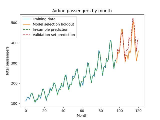
Visually, this seems pretty good - our model seems to capture the long-term trend and cyclic structure of the data. However, our choice of $p=5$ was a guess; perhaps a more or less complex model (that is, a model with more or fewer lag terms) would perform better. We’ll perform cross-validation by trying different values of $p$ with the holdout set.
from scipy.stats import sem

lag_values = np.arange(1, 40)
mse = []
error_sem = []

for p in lag_values:
    ar_model = AutoReg(endog=train_df.log_passengers, exog=train_exog, lags=p, trend='ct')
    ar_fit = ar_model.fit()

    select_log_pred = ar_fit.predict(start=select_df.t.min(), end=select_df.t.max(), exog_oos=select_exog)
    select_resid = select_df.Passengers - np.exp(select_log_pred)
    mse.append(np.mean(select_resid**2))
    error_sem.append(sem(select_resid**2))

mse = np.array(mse)
error_sem = np.array(error_sem)

plt.plot(lag_values, mse, marker='o')
plt.fill_between(lag_values, mse - error_sem, mse + error_sem, alpha=.1)
plt.xlabel('Lag Length P')
plt.ylabel('MSE')
plt.title('Lag length vs error')
plt.show()
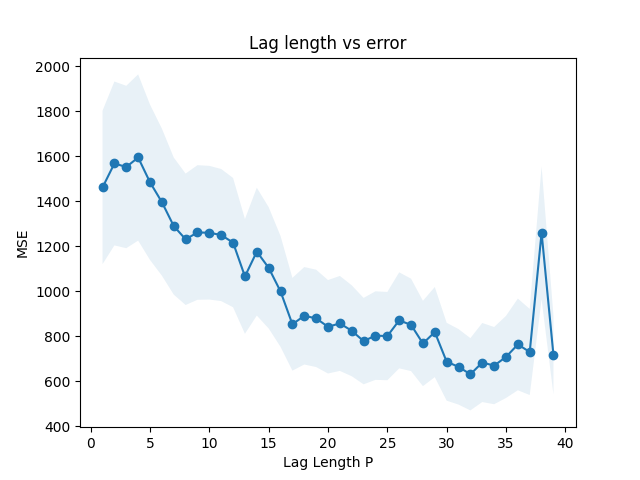
Adding more lags seems to improve the model, but has diminishing returns. We’ve computed a standard error on the average squared residual. Using the one standard error rule, we’ll pick $p=17$, the lag which is smallest but within 1 standard error of the best model.
Now that we’ve picked the lag length, let’s see whether the model assumptions hold. When we subtract out the predictions of our model, we should be left with something that looks like Gaussian white noise - errors which are normally distributed around zero, and which have no autocorrelection. Let’s start by
train_and_select_df = df[df['t'] <= validate_cutoff]
train_and_select_exog = build_design_matrices([dm.design_info], train_and_select_df, return_type='dataframe')[0]

ar_model = AutoReg(endog=train_and_select_df.log_passengers,
                   exog=train_and_select_exog, lags=17, trend='ct')
ar_fit = ar_model.fit()

plt.title('Residuals')
plt.plot(ar_fit.resid)
plt.show()
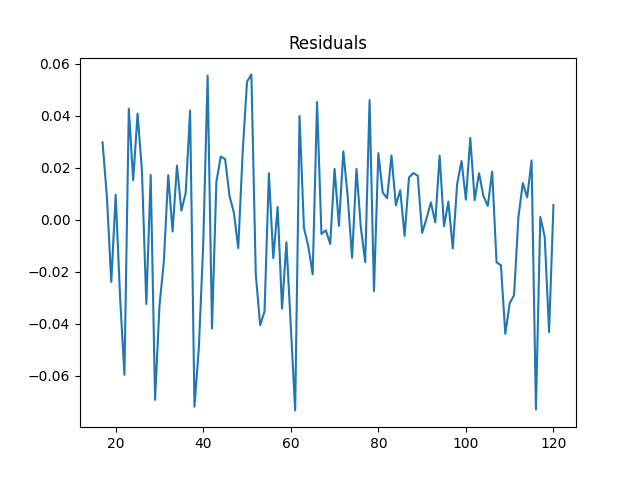
The mean residual is about zero. If I run np.mean and sem, we see that average residual is 3.2e-14, with a standard error of .003. So this does appear to be centered around zero. To see if it’s uncorrelated with itself, we’ll compute the partial autocorrelation.
from statsmodels.graphics.tsaplots import plot_pacf

plot_pacf(ar_fit.resid)
plt.show()
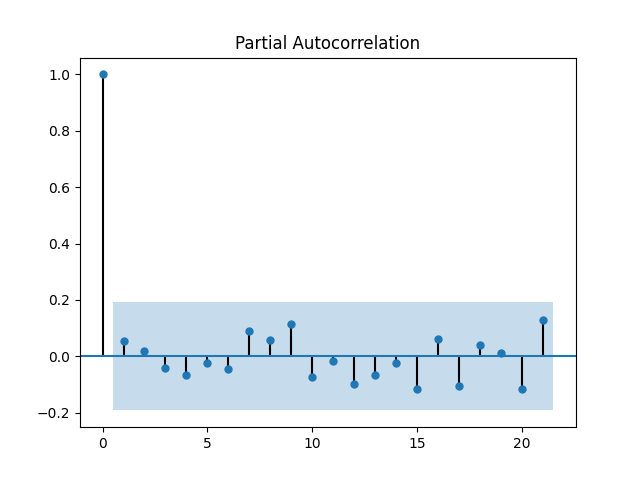
This plot is exactly what we’d hope to see - we can’t find any lag for which there is a non-zero partial autocorrelation.
Producing forecasts and prediction intervals
So far we’ve selected a model, and confirm the model assumptions. Now, let’s re-fit the model up to the forecast period, and see how we do on some new dates.
train_and_select_log_pred = ar_fit.predict(start=train_and_select_df.t.min(), end=train_and_select_df.t.max(), exog_oos=train_and_select_exog)
forecast_log_pred = ar_fit.predict(start=forecast_df.t.min(), end=forecast_df.t.max(), exog_oos=forecast_exog)

plt.plot(train_and_select_df.t, train_and_select_df.Passengers, label='Training data')
plt.plot(forecast_df.t, forecast_df.Passengers, label='Out-of-sample')
plt.plot(train_and_select_df.t,
         np.exp(train_and_select_log_pred), linestyle='dashed', label='In-sample prediction')
plt.plot(forecast_df.t,
         np.exp(forecast_log_pred), linestyle='dashed', label='Forecast')
plt.legend()
plt.title('Airline passengers by month')
plt.ylabel('Total passengers')
plt.xlabel('Month')
plt.show()
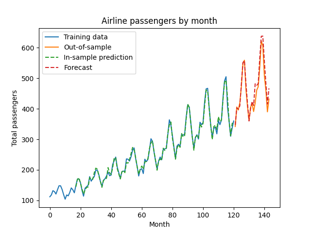
Our predictions look pretty good! Our selected model performs well when forecasting data it did not see during the training or model selection process. The predictions are arrived at recursively - so by predicting next month’s value, then using that to predict the month after that, etc. statsmodels hides that annoying recursion behind a nice interface, letting us get a point forecast out into the future.
In addition to a point prediction, it’s often useful to make an interval prediction. For example:
- In capacity planning you often want to know the largest value that might occur in the future
- In risk management you often want to know the smallest value that your investments might produce in the future
- When monitoring metrics, you might want to know whether the observed value is within the bounds of what we expect.
Because our prediction is recursive, our prediction intervals will get wider as the forecast range gets further out. I think this makes intuitive sense; forecasts of the distance future are harder than the immediate future, since errors pile up more and more as you go further out in time.
More formally, our white noise has some standard deviation, say $\sigma$. We can get a point estimate, $\hat{\sigma}$ by looking at the standard deviation of the residuals. In that case, a 95% prediction interval for the next time step is $\pm 1.96 \hat{\sigma}$. If we want to forecast two periods in the future, we’re adding two white noise steps to our prediction, meaning the prediction interval is $\pm 1.96 \sqrt{2 \hat{\sigma}^2}$ since the the variance of the sum is the sum of the variances. In general, the prediction interval for $k$ time steps in the future is $\pm 1.96 \sqrt{k \hat{\sigma}^2}$.
residual_variance = np.var(ar_fit.resid)
prediction_interval_variance = np.arange(1, len(forecast_df)+1) * residual_variance
forecast_log_pred_lower = forecast_log_pred - 1.96*np.sqrt(prediction_interval_variance)
forecast_log_pred_upper = forecast_log_pred + 1.96*np.sqrt(prediction_interval_variance)

plt.plot(train_and_select_df.t, train_and_select_df.Passengers, label='Training data')
plt.plot(forecast_df.t, forecast_df.Passengers, label='Out-of-sample')
plt.plot(train_and_select_df.t,
         np.exp(train_and_select_log_pred), linestyle='dashed', label='In-sample prediction')
plt.plot(forecast_df.t,
         np.exp(forecast_log_pred), linestyle='dashed', label='Forecast')
plt.fill_between(forecast_df.t,
        np.exp(forecast_log_pred_lower), np.exp(forecast_log_pred_upper),
        label='Prediction interval', alpha=.1)
plt.legend()
plt.title('Airline passengers by month')
plt.ylabel('Total passengers')
plt.xlabel('Month')
plt.show()
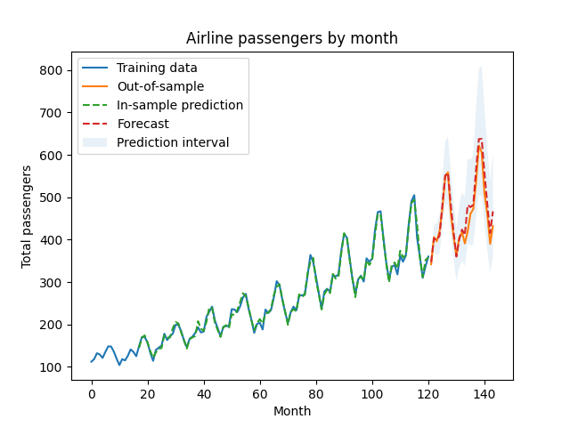
And there we have it! Our prediction intervals fully cover the observations in the forecast period; note how the intervals become wider as the forecast window gets larger.
Written on July 21st , 2021 by Louis Cialdella