Picking the model with the lowest cross validation error is not enough

We often pick the model with the lowest CV error, but this leaves out valuable information. Specifically, it ignores the uncertainty around the estimated out-of-sample error. It’s useful to calculate the standard errors of a CV score, and incorporate this uncertainty into our model selection process. Doing so avoids false precision in model selection and allows us to better balance out-of-sample error with other factors like model complexity.

We build trust in our models by demonstrating that they make good predictions on out-of-sample data. This process, called cross validation, is at the heart of most model evaluation procedures. It allows us to easily compare the performance of any black-box models, though they may have differing structures or assumptions.

Most commonly, methods like K-fold cross validation are used to compute point estimates of the model’s out-of-sample error. If you have two candidate models, cross validation will produce an estimate of how your favorite goodness-of-fit metric, like the MSE or ROC-AUC, looks for each (we’ll talk about “error” and minimizing it here, but this could easily be maximization as well). The simplest method used by practictioners to select among competing models is usually to pick the model with the lowest out-of-sample error averaged over the k folds.

Point estimates are a great start. But they’re rarely the whole story - in most other investigations, we also want a measure of the uncertainty around any estimate. In order to understand the range of potential business outcomes, this is often useful information in its own right. And without it, we might end up in a situation where two models have similar point estimates but it’s unclear if they’re significantly different. How should we compute confidence intervals around a model’s out-of-sample error? How should we use that information if we want to select a model? ¹

Standard errors for K-fold cross validation

When we run K-fold cross validations for a model specification, we end up with k point estimates of our favorite metric (MSE, ROC-AUC, accuracy, or whatever your favorite metric is). We’ll call these point estimates of the error $e_1, e_2, …, e_k$. Our combined estimate of the out-of-sample error over the k folds is usually the average of these:

In the case where k is much smaller than the dataset (in practice, we often use something like k=10), we can treat these like IID variables and compute the standard error of their mean in the usual way. With a short prayer to the assumptions of Central Limit Theorem², we can compute the standard error

And ta-da! We’ve got a quick estimate of the standard error of the out-of-sample error. ³

Model complexity vs Uncertain knowledge of prediction quality

With the ability to compute standard errors on the out-of-sample error, we can now compute confidence intervals around the estimated error. This is useful for helping us understand if the difference between two models is statistically significant, which is certainly useful. What should we do in the case where a few models seem to tie for the best spot? For example, if the top two models have out-of-sample errors that are not statistically significantly different?

One tempting option is to give up and just pick the model with the best point estimate. At least we were careful! And fair enough. In this case, we’ll get the same result as the “pick the best point estimate” strategy we started with. Another is to pick the one with the smallest worst-case error. This might make sense if the models have widely differing standard errors; it’s basically minimax approach that is conservative in the face of uncertainty.

Both of these are defensible options. They are both potentially missed opportunities, though. If we believe that we have a collection of models with prediction power that is “about the same”, as far as we can tell, we can decide between them using some other criterion that we think is important.

Specifically, when all else is equal, we prefer simpler models. In our model selection problem, that roughly translates to “if all the models have similar predictive power, pick the model which is least complex.” This is the model selection equivalent of Occam’s razor; for Bayesians, it corresponds to a prior that the “among similar explanations, the simplest explanation is probably the right one”.

How do we turn this philsophical preference for simpler models into a model selection rule? Many types of models have a parameter that controls their overall complexity. These are everywhere: the degree of a polynomial feature, the degrees of freedom of a spline, the regularization strength in a Ridge or LASSO model, the pruning parameter in a tree, the size of a neural network’s hidden layer, etc. We can then turn our maxim into a more actionable command: “Among competing models with similar out-of-sample error, pick the one with the smallest complexity.”

Hastie, Tibshirani, and Friedman define a heuristic for doing this that they call the “one standard error rule”. They suggest performing K-fold cross validation, and taking the model with the lowest complexity which is within one standard error of the best-performing model’s CV score. ⁴ For them (the venerable originators of the LASSO), their measure of complexity is the regularization strength in their model. This often produces a model which produces “about the same” quality of prediction as the best-performing model, but usually is substantially simpler. There’s no reason to limit this to just conversations about the LASSO, though - it seems to me like any model class that has a complexity parameter could be chosen this way. ⁵

Putting it all together: CIs and the one standard error rule for Sklearn models

As always, scikit-learn is there to do the hard work for us. It turns out we don’t have to write much extra code to compute these CIs from the cross validation tools and use them to apply the one standard error rule.

We’ll use a wine quality dataset that I found on the UCI Data Set Library. Our goal is to predict the quality of the wine (measured on a numeric scale) when given various laboratory measurements of its composition. We’ll apply the one standard error rule to select a LASSO model for this data.

First, we’ll grab the data:

curl http://www3.dsi.uminho.pt/pcortez/wine/winequality.zip --output winequality.zip
unzip winequality.zip
cd winequality/

And import the usual suspects so we can read in the data:

from sklearn.tree import DecisionTreeRegressor
from sklearn.linear_model import Lasso
from sklearn.model_selection import cross_val_score
import numpy as np
from matplotlib import pyplot as plt
import seaborn as sns
from sklearn.preprocessing import StandardScaler
import pandas as pd

df = pd.read_csv('winequality-red.csv', sep=';')

y = df['quality']
X = df.drop('quality', axis=1)

In this case, the complexity is governed by the alpha parameter. The larger the alpha, the less complex the model. We’ll start by picking some candidate values of alpha in a predefined range:

candidate_alpha = [10**i for i in np.linspace(-5, -2, 200)]
candidate_regressors = [Lasso(alpha=a, normalize=True) for a in candidate_alpha]

Remember, alpha should be positive, and more alpha means more regularization. Here I limited it to a range of values that produce reasonable cross-validation results to illustrate the method; I initially searched a wider range (not shown).

We’ll run a 10-fold cross validation for each choice of alpha, and compute the standard error of the MSE for each model.

cv_results = [-cross_val_score(r, X, y, scoring='neg_root_mean_squared_error', cv=10) for r in candidate_regressors]
cv_means = np.array([np.mean(cv) for cv in cv_results])
cv_se = np.array([np.std(cv) / np.sqrt(10) for cv in cv_results])

We’ll pick two models from this set of cross validations. We’ll grab the index of the model with the lowest average error (min_i) as well as the model we would select using the one standard error rule (one_se_i).

min_i = np.argmin(cv_means)
cutoff = cv_means[min_i] + cv_se[min_i]

one_se_rule_i = np.argmax(candidate_alpha * (cv_means < cutoff))

Let’s plot the estimated MSE of all the models we tried with their standard errors, highlighting the two models we picked.

plt.plot(candidate_alpha, cv_means)
plt.fill_between(candidate_alpha, cv_means + 1*cv_se, cv_means - 1*cv_se, alpha=.1)
plt.axhline(cutoff, linestyle='dotted', label='Best + One SE')
plt.scatter([candidate_alpha[one_se_rule_i]], [cv_means[one_se_rule_i]], marker='o', color='orange', label='One SE Rule')
plt.scatter([candidate_alpha[min_i]], [cv_means[min_i]], marker='o', color='blue', label='Minimum rule')
plt.legend()
plt.xscale('log')
plt.xlabel('Log alpha')
plt.ylabel('MSE')
plt.show()

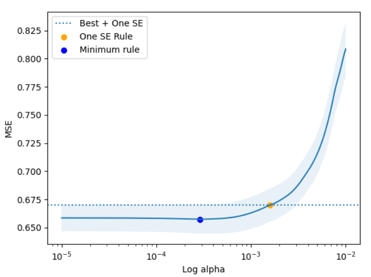
This plot provides a valuable bit of intuition about a pattern that often shows up when building models. Often there is a point where the model is “maxed out” - where adding additional model complexity doesn’t seem to get us much in terms of reduced error. The one SE rule allows us to pick a model which has similar predictive power but may be much simpler than other models. In this example, we see that we end up picking a model with meaningfully more regularization. To make that concrete, the minimum error model (blue) has 7 coeffiicients, but the one SE rule model is much sparser, having only 4.

What else might we do with this? Multiple comparisons and hierarchical models

The one SE rule is a useful model selection rule. There are other ways we might imagine using the information about uncertainty in model performance:

• We might think of comparing a bunch of models to understand which ones are statistically significantly better than the others, or at least better than the baseline. If we do so, though, we’ll need to ensure we do a bunch of multiple testing corrections.
• We could think about each model’s cross validation error as a hierarchical model. That is, errors on individual predictions are drawn from the distribution of errors in a given fold, and each fold’s parameters are drawn from the distribution of the model’s errors. This might even lead to a pleasant framework for incorporating K-fold cross validation into a framework for Bayesian optimization.

Endnotes

1: A helpful reference, from which a number of these ideas were adapted directly, are the lecture notes for Stanford’s Data Mining: 36-462/36-662 with Rob Tibshirani. These notes and these notes in particular are useful, as is section 7.10 of ESL.

2: Specifically, that the data are independent and the finite-sample distribution of the mean is normal. When k=10, these seem reasonably mild as assumptions go. A sample size of 10 is often enough for “well behaved” data like MSE, though you can play around with this to confirm your intuition. The random splitting might allow us to claim independence, though this becomes a trickier assumption as k gets large. By the time we get to the Leave-one-out case, for example, it should be clear that each datapoint’s predictions are highly correlated.

3: The method here is the one given in the lecture notes and ESL; the k averages are treated as data and we use our usual standard error formula. It seems possible that this understates the variance. For example, it seems reasonable to compute the SE for the error metric on each of the K datasets (perhaps by bootstrap) and then computing the SE of the combined metric over the k folds. I haven’t found a reference that does this yet, though.

4: It is not clear to me what justifies the use of one standard error specifically, but it operationalizes the Occam-y idea that we want “the simplest model that makes good predictions”. Even if it’s not obvious that it’s optimal, it seems like a very useful heuristic.

5: This method would need some additions to account for comparisons between model types - for example, if we wanted to compare a decision tree and a linear model, it’s not immediately clear which is more complex.

Within a single type of model, though, it’s pretty general. Here’s an example of using the one standard error rule to select a tree instead of a LASSO model:

candidate_alpha = np.linspace(0, 0.1, 200)
candidate_regressors = [DecisionTreeRegressor(ccp_alpha=a) for a in candidate_alpha]

cv_results = [-cross_val_score(r, X, y, scoring='neg_root_mean_squared_error', cv=10) for r in candidate_regressors]
cv_means = np.array([np.mean(cv) for cv in cv_results])
cv_se = np.array([np.std(cv) / np.sqrt(10) for cv in cv_results])

min_i = np.argmin(cv_means)
cutoff = cv_means[min_i] + cv_se[min_i]

one_se_rule_i = np.argmax(candidate_alpha * (cv_means < cutoff))

plt.plot(candidate_alpha, cv_means)
plt.fill_between(candidate_alpha, cv_means + 1*cv_se, cv_means - 1*cv_se, alpha=.1)
plt.axhline(cutoff, linestyle='dotted', label='Best + One SE')
plt.scatter([candidate_alpha[one_se_rule_i]], [cv_means[one_se_rule_i]], marker='o', color='orange', label='One SE Rule')
plt.scatter([candidate_alpha[min_i]], [cv_means[min_i]], marker='o', color='blue', label='Minimum rule')
plt.legend()
plt.xlabel('Alpha')
plt.ylabel('MSE')
plt.show()