The False-Discovery Rate: An alternative to the FWER for multiple comparisons

We’ve previously explored one common method for dealing with testing multiple simultaneous hypotheses, methods that control the Family-wise error rate. However, we realized that the FWER can be quite conservative. The False-Discovery rate is a powerful alternative to the FWER, which is often used in cases where hundreds or thousands of simultaneous hypotheses are tested. What is the FDR, and how is it different from the FWER? How do we control it?

What happens to the FWER when we test hundreds or thousands of hypotheses?

In our discussion of the FWER, we walked through some strategies for avoiding Type I errors when we test multiple simulataneous hypotheses. It turned out that when we tested 5 hypotheses instead of one, we might accidentally reject a true null hypothesis much more often than $\alpha$, our significant level. We looked at the Bonferroni and Bonferroni-Holm methods, which let us ensure that the probabilty of any false claims at all was less than $\alpha$.

Let’s imagine a scenario where instead of testing 5 hypotheses, we’re testing 5000. While this might seem a little far fetched, it occurs pretty frequently:

• Machine learning models might have hundreds or thousands of features which we’d like to test for their correlation with the output
• Microarray studies involve looking at the expression of thousands of genes
• Experiments might cast a wide net and screen many possible treatments for potential value

In a case like this, our analysis might produce a giant number of significant results. An experiment which screens thousands of potential treatments might involve rejecting hundreds of null hypotheses. If that’s the case, the FWER is pretty strict - it will ensure that we very rarely make even one false statement. But in a lot of these cases, we’re intentionally casting a wide net, and we don’t need to be so conservative. We’re often perfectly happy to reject 250 null hypotheses when we should have only rejected 248 of them; we still found 248 new and exciting relationships we can explore! The FWER-controlling methods, though, will work hard to make sure this doesn’t happen. If we’re very sensitive to False Positives, FWER control is what we need - but often with many hypotheses, it’s not what we’re looking for.

The goal of FDR control: Make sure few of your findings are spurious

The FWER, it turns out, is just one way of thinking about the Type I error rate when we test multiple hypotheses. In the case above, we had two false positives; but we had so many true positives that it wasn’t an especially big deal. The idea is that we made 248 “authentic” discoveries, and 2 “false” discoveries. In cases where we have so many useful discoveries, we’re often willing to pay the penalty of a few false ones. This is main idea behind controlling the False Discovery Rate, or FDR; we’d like to make it unlikely that too many of our claims are false.

Let’s get a little more specific in defining the FDR. For every hypothesis, there are four outcomes:

• A null hypothesis could be true, but we reject it, claiming a discovery when there is none. This is a False Positive.
• A null hypothesis could be false, and we reject it, claiming a discovery when there is one, hooray! This is a True Positive.
• A null hypothesis could be false, and we fail to reject it, missing out on a discovery we could have made. This is a False Negative.
• A null hypothesis could be true, and we fail to reject it, avoiding claiming a discovery when there isn’t one. This is a True Negative.

This is a bit of a mouthful, so we often summarize the four possible outcomes in a matrix like the following:

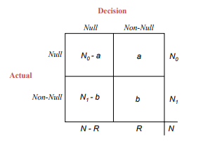
Table from the excellent Computer Age Statistical Inference, Ch. 15. My explanation glosses over some details around the definition of the FDR, and the original chapter is well worth a read.

• There are $N$ hypotheses overall. (We know this when we set up our analysis.)
• There are $N_0$ hypotheses for which the null is true, and $N_1$ hypotheses for which the alternative is true. (We don’t know this when we set up our experiment.)
• There are $a$ False positives and $b$ True positives. (We don’t know this either.)

We can use this matrix to define the FWER and FDR in terms of the decisions and results under different kinds of procedures:

• FWER-controlling methods attempt to keep $\frac{a}{N_0 + N_1} \leq \alpha$
• FDR-controlling methods attempt to keep the average $\frac{a}{a + b}$ at $\alpha$. That is, they make is so that $\mathbb{E}[\frac{a}{a + b}] = \alpha$.

Whether you decide to control the FDR or the FWER is driven by what you’d like to get our of your analysis - they solve different problems, so neither is automatically better. If you’re extremely sensitive to False Positives, then controlling the FWER might make sense; if you have many hypotheses and are willing to tolerate a small fraction of false discoveries then you might choose to control the FDR instead.

The classic method of controlling the FDR: Benjamini-Hochberg

The most well-known method of controlling the FDR is the Benjamini-Hochberg procedure. The procedure is quite similar to the Bonferroni-Holm method we discussed before. It goes something like this:

• Sort all the P-values you computed from your tests in ascending order. We’ll call these $P_1, …, P_m$, and they’ll correspond to hypotheses $H_1, …, H_m$.
• We’ll define a series of significance levels $\alpha_1, …, \alpha_m$, where $\alpha_i = \frac{\alpha \times i}{m}$.
• Starting with $P_1$, see if it is significant at the level of $\alpha_1$. If it is, reject it and move on to testing $P_2$ at $\alpha_2$. Continue until you find a hypothesis you can’t reject, and stop there.
• Put another way: If $k$ is the first index such that we can’t reject $H_k$, then reject all the hypotheses from $1, …, k-1$.

If you’d like to go a little deeper, the original 1995 paper remains pretty accessible.

The details of the method don’t need to be implemented, luckily; we simply need to call the multipletests method from statsmodels, and select fdr_bh as the method. That will tell us which of the hypotheses we entered can be rejected while keeping the FDR at the specified level.

Alternatives to the Benjamini-Hochberg procedure and related methods

The Benjamini-Hochberg procedure assumes that the hypotheses are independent. In some cases, this is clearly untrue; in others, it’s not as obvious. Nonethless, it appears that empirically the BH procedure is relatively robust to this assumption. An alternative which does not make this assumption is Benjamini–Yekutieli, but the power of this procedure can be much lower. If you’re not sure which to use, it might be worth running a simulation to compare them.

A close relative of the FDR is the False coverage rate, its confidence interval equivalent. Once we have performed the BH procedure to control the FDR, we can then compute adjusted confidence intervals for the parameters for which we rejected the null hypothesis.

An example: Feature selection in a linear model simulation

Let’s look at a concrete example. We’ll look at a large number of simulations in which we’re attempting to figure out which regression coefficients are non-zero in a linear model. In each simulation there will be 1000 covariates and 2000 samples. Of those, 100 covariates will be non-zero; the rest will be red herrings. So in each simulation we’ll run 100 simultaneous T-tests using statsmodels.

We’ll run 1000 simulations like the following:

• Generate a dataset from a linear model with 1000 covariates, of which 100 are non-zero.
• Run an OLS regression and compute P-values for each covariate using statsmodels.
• Declare some covariates significant others non-significant using the naive method (any $p < .05$ is rejected) and the Benjamini-Hochberg method.
• Calculate incorrectly discovered covariates / total discovered covariates, the False Discovery Rate.

This will give us 1000 simulations of the FDR under each procedure, and show us whether our method works.

from sklearn.datasets import make_regression
from statsmodels.api import OLS
import numpy as np
from statsmodels.stats.multitest import multipletests
from tqdm import tqdm
from matplotlib import pyplot as plt
import seaborn as sns

def simulate_fdr():
  n_tests = 1000
  n_sample = 2000
  n_true_pos = 100

  alpha = .05

  X, y, coef = make_regression(n_samples=n_sample, n_features=n_tests, n_informative=n_true_pos, bias=0, coef=True, noise=200)
  p = OLS(y, X).fit().pvalues
  reject = p <= alpha
  true_null = (coef == 0)
  count_discoveries = np.sum(reject)
  count_false_discoveries = np.sum(reject & true_null)

  reject_bh = multipletests(p, method='fdr_bh', alpha=alpha)[0]
  count_discoveries_bh = np.sum(reject_bh)
  count_false_discoveries_bh = np.sum(reject_bh & true_null)

  naive_fdr = count_false_discoveries / count_discoveries
  bh_fdr = count_false_discoveries_bh / count_discoveries_bh
  return naive_fdr, bh_fdr
  
simulations = [simulate_fdr() for _ in tqdm(range(1000))]

naive_fdr_dist, bh_fdr_dist = zip(*simulations)

sns.distplot(naive_fdr_dist, label='Naive method')
sns.distplot(bh_fdr_dist, label='BH method')
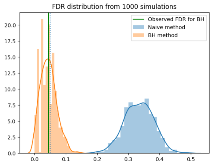
plt.title('FDR distribution from 1000 simulations')
plt.axvline(.05, linestyle='dotted')
plt.axvline(np.mean(bh_fdr_dist), label='Observed FDR for BH', color='green')
plt.legend()
plt.show()

We see that the naive method had a FDR rate of around 0.35 for this simulation - about a third of reported findings will be spurious. However, the BH procedure works as intended, keeping the FDR arond 0.05.

We mentioned that FWER-controlling methods are more conservative than FDR-controlling ones. Let’s take a look at a single simulation to explore the difference between Benjamini-Hochberg and Bonferroni-Holm in action.

sorted_p, sorted_true_null = zip(*sorted(zip(p, true_null)))
sorted_p = np.array(sorted_p)
sorted_true_discoveries = (1. - np.array(sorted_true_null)).astype(np.bool)

alpha = .05
i = np.arange(len(sorted_p)) + 1
m = len(sorted_p)
holm_cutoffs = alpha / (m + 1 - i)
hochberg_cutoffs = (alpha * i) / len(sorted_p)
plt.plot(sorted_p, label='P-values, sorted')
plt.plot(holm_cutoffs, label='Bonferroni-Holm')
plt.plot(hochberg_cutoffs, label='Benjamini-Hochberg')
plt.scatter(i[sorted_true_discoveries]-1, sorted_p[sorted_true_discoveries], marker='x')
plt.legend()
plt.show()

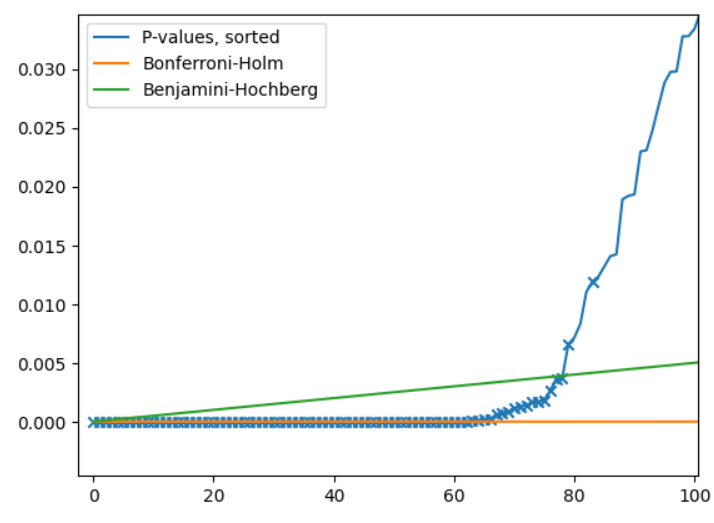
We’re only looking at the first 100 hypotheses here. The “genuine discoveries” are indicated by an X. We see that Bonferroni-Holm is much more strict than Benjamini-Hochberg. Both methods will correctly reject the “obvious” P-values very close to zero, but Bonferroni-Holm misses out on a number of discoveries because it is so strict. The hypotheses missed by Bonferroni-Holm but caught by Benjamini-Hochberg are the points with an X below the green line, but above the yellow one.

What else might we do?

We’ve repeatedly noted that FDR-controlling methods are an alternative to FWER-controlling ones. Are there any other choices we could make here?

As I mentioned in my last post, a third option is to abandon the Type I error paradigm altogether. This school of thought is (in my view) convincingly argued by Andrew Gelman. His perspective, very roughly, is that null hypotheses are usually not true anyway, and that Type I error control is not worth the price we pay for it in power. Rather, we should focus on correctly estimating the magnitude of the effects we care about, and that if we adopt a Bayesian perspective the problems go away and we can use all the available information to fit a hierarchical model and get a more realistic view of things.