Symbolic Calculus in Python: Simple Samples of Sympy

My job seems to involve just enough calculus that I can’t afford to forget it, but little enough that I always feel rusty when I need to do it. In those cases, I’m thankful to be able to check my work and make it reproducible with Sympy, a symbolic mathematics library in Python. Here are two examples of recent places I’ve used Sympy to do calculus. We’ll start by computing the expected value of a distribution by doing a symbolic definite integral. Then, we’ll find the maximum of a model by finding its partial derivatives symbolically, and setting it to zero.

Symbolic Integration: Finding the moments of a probability distribution

A simple model for a continuous, non-negative random variable is a half-normal distribution. This is implemented in scipy as halfnorm. The scipy version is implemented in terms of a scale parameter which we’ll call $s$. If we’re going to use this distribution, there are a few questions we’d like to answer about it:

• What are the moments of this distribution? How do the mean and variance of the distribution depend on $s$?
• How might we estimate $s$ from some data? If we knew the relationship between the first moment and $s$, we could use the Method of Moments for this univariate distribution.

Scipy lets us do all of these numerically (using functions like mean(), var(), and fit(data)). However, computing closed-form expressions for the above gives us some intuition about how the distribution behaves more generally, and could be the starting point for further analysis like computing the standard errors of $s$.

The scipy docs tell us that the PDF is:

$f(x) = \frac{1}{s} \sqrt{\frac{2}{\pi}} exp(\frac{-\frac{x}{s}^2}{2})$

Computing the mean of the distribution requires solving an improper integral:

$\mu = \int_{0}^{\infty} x f(x) dx$

Similarly, finding the variance requires doing some integration:

$\sigma^2 = \int_{0}^{\infty} (x - \mu)^2 f(x) dx$

We’ll perform these integrals symbolically to learn how $s$ relates to the mean and variance. We’ll then rearrange $s$ in terms of $\mu$ to get an estimating equation for $s$.

We’ll import everything we need:

import sympy as sm
from scipy.stats import halfnorm
import numpy as np

Variables which we can manipulate algebraically in Sympy are called “symbols”. We can instantiate one at a time using Symbol, or a few at a time using symbols:

x = sm.Symbol('x', positive=True)
s = sm.Symbol('s', positive=True)

# x, s = sm.symbols('x s') # This works too

We’ll specify the PDF of scipy.halfnorm as a function of $x$ and $s$:

f = (sm.sqrt(2/sm.pi) * sm.exp(-(x/s)**2/2))/s

It’s now a simple task to symbolically compute the definite integrals defining the first and second moments. The first argument to integrate is the function to integrate, and the second is a tuple (x, start, end) defining the variable and range of integration. For an indefinite integral, the second argument is just the target variable. Note that oo is the cute sympy way of writing $\infty$.

mean = sm.integrate(x*f, (x, 0, sm.oo))

var = sm.integrate(((x-mean)**2)*f, (x, 0, sm.oo))

And just like that, we have computed closed-form expressions for the mean and variance in terms of $s$. You could use the LOTUS to calculate the EV of any function of a random variable this way, if you wanted to.

Printing sm.latex(mean) and sm.latex(var), we see that:

$\mu = \frac{\sqrt{2} s}{\sqrt{\pi}}$

$\sigma^2 = - \frac{2 s^{2}}{\pi} + s^{2}$

Let’s make sure our calculation is right by running a quick test. We’ll select a random value for $s$, then compute its mean/variance symbolically as well as using Scipy:

random_s = np.random.uniform(0, 10)

print('Testing for s = ', random_s)
print('The mean computed symbolically', mean.subs(s, random_s).subs(sm.pi, np.pi).evalf(), '\n',
      'The mean from Scipy is:', halfnorm(scale=random_s).mean())
print('The variance computed symbolically', var.subs(s, random_s).subs(sm.pi, np.pi).evalf(), '\n',
      'The variance from Scipy is:', halfnorm(scale=random_s).var())

Testing for s =  3.2530297154660213
The mean computed symbolically 2.59554218580328
 The mean from Scipy is: 2.595542185803277
The variance computed symbolically 3.84536309142049
 The variance from Scipy is: 3.8453630914204933

It looks like our expressions for the mean and variance are correct, at least for this randomly chosen value of $s$. Running it a few more times, it looks like it works more generally.

Symbolic Differentiation: Finding the maximum of a response surface model

Sympy also lets us perform symbolic differentiation. Unlike numerical differentiation and automatic differentiation, symbolic differentiation lets us compute the closed form of the derivative when it is available.

Imagine you are the editor of an email newsletter for an ecommerce company. You currently send out newsletters with two types of content, in the hopes of convinncing customers to spend more with your business. You’ve just run an experiment where you change the frequency at which newsletters of each type are sent out. This experiment includes two variables:

• $x$, the change from the current frequency in percent terms for email type 1. In the experiment this varied in the range $[-10\%, 10\%]$, as you considered an increase in the frequency as large as 10% and a decrease of the same magnitude.
• $y$, the change from the current frequency in percent terms for email type 2. This also was varied in the range $[-10\%, 10\%]$.

In your experiment, you tried a large number of combinations of $x$ and $y$ in the range $[-10\%, 10\%]$. You’d like to know: based on your experiment data, what frequency of email sends will maximize revenue? In order to learn this, you fit a quadratic model to your experimental data, estimating the revenue function $r$:

$r(x, y) = \alpha + \beta_x x + \beta_y y + \beta_{x2} x^2 + \beta_{y2} y^2 + \beta_{xy} xy$

We can now learn where the maxima of the function are, doing some basic calculus.

Again, we start with our imports:

import sympy as sm
from matplotlib import pyplot as plt
from sklearn.utils.extmath import cartesian
import numpy as np
import matplotlib.ticker as mtick

Next, we define symbols for the model. We have the experiment variables $x$ and $y$, plus all the free parameters of our model, and the revenue function.

x, y, alpha, beta_x, beta_y, beta_xy, beta_x2, beta_y2 = sm.symbols('x y alpha beta_x beta_y beta_xy beta_x2 beta_y2')

rev = alpha + beta_x*x + beta_y*y + beta_xy*x*y + beta_x2*x**2 + beta_y2*y**2 

We’ll find the critical points by using the usual method from calculus, that is by finding the points where $\frac{dr}{dx} = 0$ and $\frac{dr}{dy} = 0$.

critical_points = sm.solve([sm.Eq(rev.diff(var), 0) for var in [x, y]], [x, y])

print(sm.latex(critical_points[x]))
print(sm.latex(critical_points[y]))

We find that the critical points are:

$x_* = \frac{- 2 \beta_{x} \beta_{y2} + \beta_{xy} \beta_{y}}{4 \beta_{x2} \beta_{y2} - \beta_{xy}^{2}}$ $y_* = \frac{\beta_{x} \beta_{xy} - 2 \beta_{x2} \beta_{y}}{4 \beta_{x2} \beta_{y2} - \beta_{xy}^{2}}$

This gives us the general solution - if we estimate the coefficients from our data set, we can find the mix that maximizes revenue.

Let’s say that we fit the model from the data, and that we got the following estimated coefficient values:

coefficient_values = [
(alpha, 5),
(beta_x, 1), 
(beta_y, 1), 
(beta_xy, -1), 
(beta_x2, -10), 
(beta_y2, -10)
]

We substitute the estimated coefficients into the revenue function:

rev_from_experiment = rev.subs(coefficient_values)

That code generated a symbolic function. Let’s use it to create a numpy function which we can evaluate quickly using lambdify:

numpy_rev_from_experiment = sm.lambdify((x, y), rev_from_experiment)

Then, we’ll plot the revenue surface over the experiment space, and plot the maximum we found analytically:

plt.gca().yaxis.set_major_formatter(mtick.PercentFormatter(1))
plt.gca().xaxis.set_major_formatter(mtick.PercentFormatter(1))

x_y_pairs = cartesian([np.linspace(-.1, .1), np.linspace(-.1, .1)])
z = [numpy_rev_from_experiment(x_i, y_i) for x_i, y_i in x_y_pairs]

x_plot, y_plot = zip(*x_y_pairs)

plt.tricontourf(x_plot, y_plot, z)
plt.colorbar(label='Revenue per user')

x_star = critical_points[x].subs(coefficient_values)
y_star = critical_points[y].subs(coefficient_values)
plt.scatter([x_star], [y_star], marker='x', label='Revenue-maximizing choice')

plt.xlabel('Change in frequency of email type 1')
plt.ylabel('Change in frequency of email type 2')
plt.title('Revenue surface from experimental data')
plt.tight_layout()
plt.legend()
plt.show()

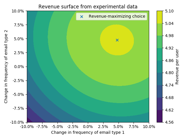
And there you have it! We’ve used our expression for the maximum of the model to find the value of $x$ and $y$ that maximizes revenue. I’ll note here that in a full experimental analysis, you would want to do more than just this: you’d also want to check the specification of your quadratic model, and consider the uncertainty around the maximum. In practice, I’d probably do this by running a Bayesian version of the quadratic regression and getting the joint posterior of the critical points. You could probably also do some Taylor expanding to come up with standard errors for these, if you wanted to do even more calculus.