Machine learning models for decision making in Python: Picking thresholds for asymmetric payoffs

Machine learning practitioners spend a lot of time thinking about whether their model makes good predictions, usually in the form of checking calibration, accuracy, ROC-AUC, precision or recall. But for ML to add value, its predictions need to be harnessed for decision making, not just prediction. We’ll walk through how you can use probabilistic classifiers not just to make accurate predictions, but to make decisions that lead to the best outcomes.

Machine learning gives us a prediction, which we use to make a decision

Lots of use cases for ML classifiers in production involve using the classifier to predict whether a newly observed instance is in the class of items we would like to perform some action on. For example:

• Systems which try to detect irrelevant content on platforms do so because we’d like to limit the distribution of this content.
• Systems which try to detect fraudulent users do so because we’d like to ban these users.
• Systems which try to detect the presence of treatable illnesses do so because we’d like to refer people with illnesses for further testing or treatment.

In all of these cases, there are two classes: a class that we have targeted for treatment (irrelevant content, fraudulent users, people with treatable illnesses), and a class that we’d like to leave alone (relevant content, legitimate users, healthy people). Some systems choose between more than just these two options, but let’s keep things simple for now. It’s common to have a workflow that goes something like this:

1. Train the model on historical data. The model will compute the probability that an instance is in the class targeted for treatment.
2. Observe the newest instance we want to make a decision about.
3. Use our model to predict the probability that this instance belongs to the class we have targeted for action.
4. If the probability that the instance is in the targeted class is greater than $\frac{1}{2}$, apply the treatment.

The use of $\frac{1}{2}$ as a threshold is a priori pretty reasonable - we’ll end up predicting the class that is more likely for a given instance. It’s so commonly used that it’s the default for the predict method in scikit-learn. However, in most real life situations, we’re not just looking for a model that is accurate, we’re looking for a model that helps us make a decision. We need to consider the payoffs and risks of incorrect decisions, and use the probability output by the classifier to make our decision. The main question will be something like: “How do we use the output of a probabilistic classifier to decide if we should take an action? What threshold should we apply?”. The answer, it turns out, will depend on whether or not your use case involves asymmetric risks.

A prototypical example: Disease detection

Assume we’ve used our favorite library to build a model which predicts the probability that an individual has a malignant tumor based on some tests we ran. We’re going to use this prediction to decide whether we want to refer the patient for a more detailed test, which is more accurate but more costly and invasive. Following tradition, we refer to the test data as $X$ and the estimated probability of a malignant tumor as $\hat{y}$. We think, based on cross-validation, that our model proves a well-calibrated estimate of $\mathbb{P}(Cancer \mid X) = \hat{y}$. For some particular patient, we run their test results ($X$) through our model, and compute their probability of a malignant tumor, $\hat{y}$. We’ve used our model to make a prediction, now comes the decision: Should we refer the patient for further, more accurate (but more invasive) testing?

There are four possible outcomes of this process:

• We refer the patient for further testing, but the second test reveals the tumor is benign. This means our initial test provided a false positive (FP).
• We refer the patient for further testing, and the second test reveals the tumor is malignant. This means our initial test provided a true positive (TP).
• We decline to pursue further testing. Unknown to us, the second test would have shown the tumor is benign. This means our initial test provided a true negative (TN).
• We decline to pursue further testing. Unknown to us, the second test would have shown the tumor is malignant. This means our initial test provided a false negative (FN).

We can group the outcomes into “bad” outcomes (false positives, false negatives), as well as “good” outcomes (true positives, true negatives). However, there’s a small detail here we need to keep in mind - not all bad outcomes are equally bad. A false positive results in costly testing and psychological distress for the patient, which is certainly an outcome we’d like to avoid; however, a false negative results in an untreated cancer, posing a risk to the patient’s life. There’s an important asymmetry here, in that the cost of a FN is much larger than the cost of a FP.

Let’s be really specific about the costs of each of these outcomes, by assigning a score to each. Specifically, we’ll say:

• In the case of a True Negative (correctly detecting that there is no illness), nothing has really changed for the patient. Since this is the status quo case, we’ll assign this outcome a score of 0.
• In the case of a True Positive (correctly detecting that there is illness), we’ve successfully found someone who needs treatment. While such therapies are notoriously challenging for those who endure them, this is a positive outcome for our system because we’re improving the health of people. We’ll assign this outcome a score of 1.
• In the case of a False Positive (referring for more testing, which will reveal no illness), we’ve incurred extra costs of testing and inflicted undue distress on the patient. This is a bad outcome, and we’ll assign it a score of -1.
• In the case of a False Negative (failing to refer for testing, which would have revealed an illness), we’ve let a potentially deadly disease continue to grow. This is a bad outcome, but it’s much worse than the previous one. We’ll assign it a score of -100, reflecting our belief that it is about 100 times worse than a False Positive.

We’ll write each of these down in the form of a payoff matrix, which looks like this:

The matrix here has the same format as the commonly used confusion matrix. It is written (in this case) in unitless “utility” points which are relatively interpretable, but for some business problems we could write the matrix in dollars or another convenient unit. This particular matrix implies that a false negative is 100 times worse than a false positive, but that’s based on nothing except my subjective opinion. Some amount of subjectivity (or if you prefer, “expert judgement”) is usually required to set the values of this matrix, and the values are usually up for debate in any given use case. We’ll come back to the choice of specific values here in a bit.

We can now combine our estimate of malignancy probability ($\hat{y}$) with the payoff matrix to compute the expected value of both referring the patient for testing and declining future testing:

What value of $\hat{y}$ is large enough that we should refer the patient for further testing? That is - what threshold should we use to turn the probabilistic output of our model into a decision to treat? We want to send the patient for testing whenver $\mathbb{E}[\text{Send for testing}] \geq \mathbb{E}[\text{Do not test}]$. So we can set the two expected values equal, and find the point at whch they cross to get the threshold value, which we’ll call $y_*$:

\(2 y_* - 1 = -100 y_*\) \(\Rightarrow y_* = \frac{1}{102}\)

So we should refer a patient for testing whenever $\hat{y} \geq \frac{1}{102}$. This is very different than the aproach we would get if we used the default classifier threshold, which in scikit-learn is $\frac{1}{2}$.

Picking the best threshold and evaluating out-of-sample decision-making in Python

We can do a little algebra to show that if we know the 2x2 payoff matrix, then the optimal threshold is:

$y_* = \frac{\text{TN value - FP value}}{\text{TP value + TN value - FP value - FN value}}$

Let’s compute this threshold and apply it to the in-sample predictions in Python:

from sklearn.datasets import load_breast_cancer
from sklearn.linear_model import LogisticRegression
import numpy as np
from matplotlib import pyplot as plt

payoff = np.array([[0, -1], [-100, 1]])

X, y = load_breast_cancer(return_X_y=True)
y = 1-y # In the original dataset, 1 = Benign

model = LogisticRegression(max_iter=10000)
model.fit(X, y)

y_threshold = (payoff[0][0] - payoff[0][1]) / (payoff[0][0] + payoff[1][1] - payoff[0][1] - payoff[1][0])

send_for_testing = model.predict_proba(X)[:,1] >= y_threshold

Does the $y_*$ we computed lead to optimal decision making on this data set? Let’s find out by computing the average out-of-sample payoff for each threshold:

# Cross val - show that the theoretical threshold is the best one for this data

from sklearn.metrics import confusion_matrix
from sklearn.model_selection import cross_val_predict

y_pred = cross_val_predict(LogisticRegression(max_iter=10000), X, y, method='predict_proba')[:,1]

thresholds = np.linspace(0, .95, 1000)
avg_payoffs = []

for threshold in thresholds:
  cm = confusion_matrix(y, y_pred > threshold)
  avg_payoffs += [np.sum(cm * payoff) / np.sum(cm)]

plt.plot(thresholds, avg_payoffs)
plt.title('Effect of threshold on average payoff')
plt.axvline(y_threshold, color='orange', linestyle='dotted', label='Theoretically optimal threshold')
plt.xlabel('Threshold')
plt.ylabel('Average payoff')
plt.legend()
plt.show()

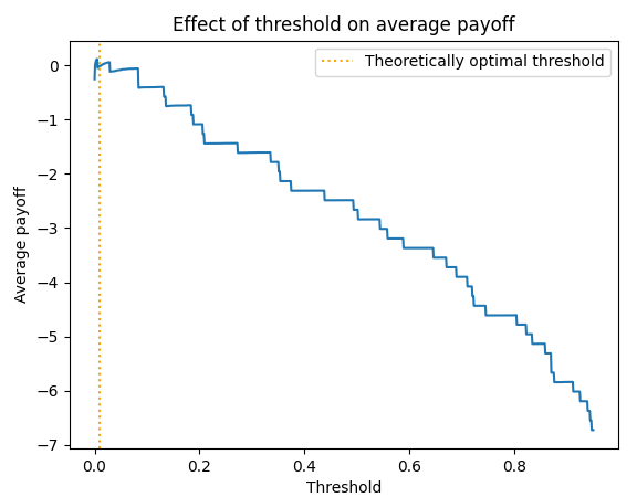
Our $y_*$ is very close to optimal on this data set. It is much better in average payoff terms than the sklearn default of $\frac{1}{2}$.

Note that in the above example we calculate the out-of-sample confusion matrix cm, and estimate the average out-of-sample payoff as np.sum(cm * payoff) / np.sum(cm). We could also use this as a metric for model selection, letting us directly select the model that makes the best decisions on average.

When is the optimal threshold $y_* = \frac{1}{2}?$

In the cancer example above, we may think it’s more likely than not that the patient is healthy, yet still refer them for testing. Because the cost of a false negative is so large, the optimal behavior is to act conservatively, recommending testing in all but the most clear-cut cases.

How would things be different if our goal was simply to make our predictions as accurate as possible? In this case we might imagine a payoff matrix like

For this payoff matrix, we are awarded a point for each correct prediction (TP or TN), and no points for incorrect predictions (FP or FN). IF we do the math for this payoff matrix, we see that $y_* = \frac{1}{2}$. That is, the default threshold of $\frac{1}{2}$ makes sense when we want to maximize the prediction accuracy, and there are no asymmetric payoffs. Other “accuracy-like” payoff matrices like

or perhaps

also have $y_* = \frac{1}{2}$.

You might at this point wonder whether the $y_* = \frac{1}{2}$ threshold also maximizes other popular metrics under symmetric payoffs, like precision and recall. We can define a “precision” payoff matrix (1 point for true positives, -1 point for false positives, 0 otherwise) as something like

If we plug $P_{precision}$ into the formula from before, we see that $y_* = \frac{1}{2}$ in this case too.

Repeating the exercise for a “recall-like” matrix (1 point for true positives, -1 point for false negatives, 0 otherwise):

This yields something different - for this matrix, $y_* = 0$. This might be initially surprising - but if we inspect the definition of recall, we see that we will not be penalized for false positives, so we might as well treat every instance we come across (this is why it’s often used in tandem with precision, which does penalize false positives).

Where do the numbers in the payoff matrix come from?

In the easiest case, we the know the values a priori, or someone has measured the effects of each outcome. If we know these values in dollars or some other fungible unit, we can plug them right into the payoff matrix. In some cases, you might be able to run an experiment, or a causal analysis, to estimate the values of the matrix. We would expect the payoffs along the main diagonal (TP, TN) to be positive or zero, and the payoffs off the diagonal (FP, FN) to be negative.

If you don’t have those available to you, or there’s no obvious unit of measurement, you can put values into the matrix which accord with your relative preferences between the outcomes. In the cancer example, our choice of payoff matrix reflected our conviction that a FN was 100x worse than a FP - it’s a statement about our preferences, not something we computed from the data. This is not ideal in a lot of ways, but such an encoding of preferences is usually much more realistic than the implicit assumption that payoffs are symmetric, which is what we get when we use the default. When you take this approach, it may be worth running a sensitivity analysis, and understanding how sensitive your ideal threshold is to small changes in your preferences.