Understanding the difference between prediction and confidence intervals for linear models in Python

The difference between prediction and confidence intervals is often confusing to newcomers, as the distinction between them is often described in statistics jargon that’s hard to follow intuitively. This is unfortunate, because they are useful concepts, and worth exploring for practitioners, even those who don’t much care for statistics jargon. This post will walk through some ways of thinking about these important concepts, and demonstrate how we can calculate them for OLS and Logit models in Python. We’ll also cover what makes the intervals wider or narrower by looking at how they’re calculated. Plus, cats in sunglasses.

Example: An OLS regression model with one independent variable

As always, it’s useful to get some intuition by looking at an example, so we’ll start with one. Let’s say that you, a serial innovator and entrepreneur, have recently started designing your very own line of that most coveted feline fashion accessory, little tiny sunglasses for cats. After the initial enormous rush of sales subsides, you sit back to consider the strategic positioning of your business, and you realize that it’s quite likely that your business is a seasonal one. Specifically, you’re pretty sure that cats are most likely to purchase sunglasses during the warm months, when they’re most likely to find themselves outdoors in need of a snappy accessory.

You collect some data on the daily temperature and dollars of sales in the region where you do most of your sales, and you plot them:

plt.scatter(df['temperature'], df['sales'], label='Observed', marker='x', color='black')
plt.xlabel('Temperature (°F)')
plt.ylabel('Sales ($)')
plt.legend()
plt.show()

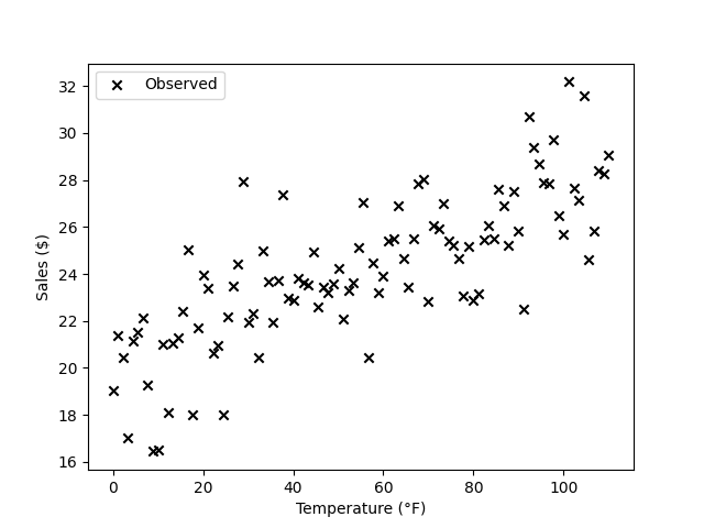
So far, so good. It looks like the two are correlated positively. In order to understand the relationship a little better, you fit yourself a line using ols:

model = smf.ols('sales ~ temperature', df)
results = model.fit()

alpha = .05

predictions = results.get_prediction(df).summary_frame(alpha)

And plot it along with the data:

plt.scatter(df['temperature'], df['sales'], label='Observed', marker='x', color='black')
plt.plot(df['temperature'], predictions['mean'], label='Regression line')
plt.xlabel('Temperature (°F)')
plt.ylabel('Sales ($)')
plt.legend()
plt.show()

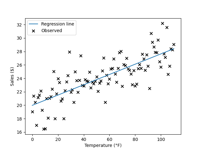
The line has a positive slope, as we expect. Of course, this is only a sample of daily temperatures, and we know that there’s some uncertainty around the particular regression line we estimated. We visualize this uncertainty by plotting the confidence interval around the predictions:

plt.fill_between(df['temperature'], predictions['mean_ci_lower'], predictions['mean_ci_upper'], alpha=.5, label='Confidence interval')
plt.scatter(df['temperature'], df['sales'], label='Observed', marker='x', color='black')
plt.plot(df['temperature'], predictions['mean'], label='Regression line')
plt.xlabel('Temperature (°F)')
plt.ylabel('Sales ($)')
plt.legend()
plt.show()

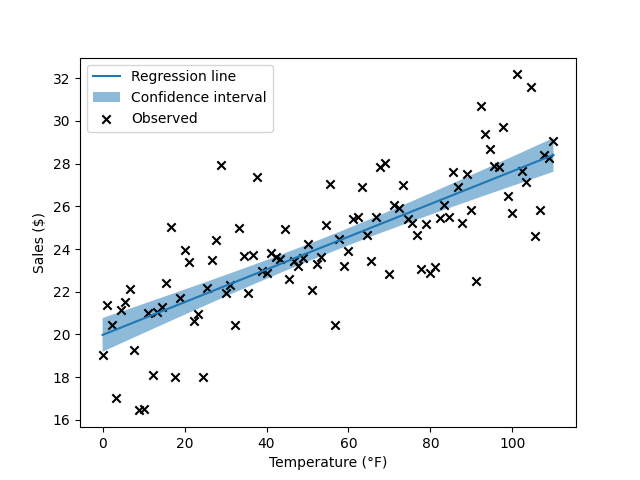
This tells us something about the uncertainty around the regression line. You’ll notice that plenty of Xs fall outside of the confidence interval. In order to visualize the region where we expect most actual sales to occur, we plot the prediction interval as well:

plt.fill_between(df['temperature'], predictions['obs_ci_lower'], predictions['obs_ci_upper'], alpha=.1, label='Prediction interval')
plt.fill_between(df['temperature'], predictions['mean_ci_lower'], predictions['mean_ci_upper'], alpha=.5, label='Confidence interval')
plt.scatter(df['temperature'], df['sales'], label='Observed', marker='x', color='black')
plt.plot(df['temperature'], predictions['mean'], label='Regression line')
plt.xlabel('Temperature (°F)')
plt.ylabel('Sales ($)')
plt.legend()
plt.show()

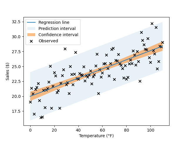
We’ve got quite a dense plot now - let’s take some time and walk through all the elements we’ve added before we tackle them in detail:

• The observed datapoints are (temperature, sales revenue) pairs.
• The regression line tells us what the average revenue is as the temperature varies in our dataset. Here, we’ve assumed that the revenue varies linearly with the temperature. The regression line answers the question: “If we know the temperature, what is our single best guess about the average level of sales we expect to see?”
• The confidence interval tells us the range of the average revenue at a given temperature. It answers the question: “If we know the temperature, what is our uncertainty around the average level of sales?”
• The prediction interval tells us the range where the observed revenue on an actual day is likely to fall at a given temperature. It answers the question: “If we know the temperature, what actual range of sales might we see on a given day?”.

Recap: What is the OLS model doing?

We can’t get into this topic without a bit of non-cat related terminology, so this section will cover that.

In this example, we had two variables: $temperature$ and $sales$. We want to know how $sales$ changes as $temperature$ varies. By convention, we often refer to the outcome we care about as $y$, and explanatory variables like $temperature$ as $x$, or perhaps $X$ if it’s a vector. We’ll assume it’s a vector going forward, because not much changes if we do.

We assume that we can write $y$ as a function of $X$, something like

The idea is that $f(X)$ tells us how the average of $y$ changes with $X$, and $\epsilon$ is a normally-distributed noise term from all the variables we didn’t choose to put in our model. If we knew the exact form of $f(X)$, we could always compute the expected value of $y$ given $X$, namely $\mathbb{E}[y \mid X] = f(X)$.

There are many choices of $f$ we could pick, but for convenience we often assume that $y$ is a linear function of $X$. In that case, we can rewrite the above expression as

Where we’ve added a vector of parameters called $\beta$ and a scalar called $\alpha$. These parameters are not known to us, but we’re going to try and estimate them from the data. There’s also another parameter, hidden in this formula - the noise term $\epsilon$ has some standard deviation, which we’ll call $\sigma$.

Running the OLS procedure, through the fit() function in statsmodels or your favorite library, computes estimates of $\alpha$, $\beta$ and $\sigma$. It also computes standard errors and p-values for those parameters. The values that we estimated from the data have that funny little hat symbol - we’ll refer to the estimates as $\hat{\alpha}$, $\hat{\beta}$ and $\hat{\sigma}$. We could similarly talk about $\hat{f}(X)$, or an estimated standard error like $\hat{SE}(\beta)$.

After we’ve estimated the model, we can compute the “average” value of $y$ given our knowledge of $X$ by computing $\hat{\alpha} + X \hat{\beta}$. So if we have a particular $X_i$ in mind, and we have not yet observed $y_i$, we can predict its expected value. We’ll call the predicted value $\hat{y_i}$, to indicate it was derived from the estimated parameter values. So for our linear model, $\hat{y_i} = \hat{\alpha} + X_i \hat{\beta}$.

Confidence intervals around the predicted mean

What does the CI for the regression line represent intuitively?

The above explanation walked through the big idea of the OLS process - we estimate $\hat{\alpha}$, $\hat{\beta}$ and $\hat{\sigma}$ from the data to get the regression line. These estimates are our “best guesses” at these values, which we sometimes call “point estimates”. As is often the case in statistics, there is some uncertainty around those estimates. This uncertainty is represented in classical statistics by confidence intervals, which are derived from the sampling distribution and standard errors. For Bayesians, the story is pretty similar - the uncertainty is represented by credible intervals, which summarize the posterior distribution.

In either case, we’re acknowledging that the point estimates $\hat{\alpha}$, $\hat{\beta}$ and $\hat{\sigma}$ leave a lot of information out. Specifically, the point estimates alone don’t tell us about how precise we think our estimates are. In addition to the point esimates we have standard errors for each one, and could compute a confidence interval for each. This uncertainty about $\hat{\alpha}$, $\hat{\beta}$ and $\hat{\sigma}$ translates into some uncertainty about the predicted value $\hat{y}$. Let’s look once more at the graph from our example:

The blue line is the regression line, our point estimate - our single best guess about the average relationship between X and y. It tells us $\hat{y}$ for every $X$. However, there are a range of regression lines that seem plausible given the data, even if they are not the absolute best fit. This range of plausible regression lines appears as the CI on the chart, the orange band around the blue regression line. Note that the CI is wider around the edges of the data set, and narrower in the middle. That is, we’re less sure about the value of $\hat{y}$ near the edges of the data set. In the notation we used before, when we said $y = f(X) + \epsilon$, the CI indicates that there are a number of different $\hat{f}(X)$ that fit the data.

To go back to our example, if we know the temperature is 40°F, we can see that the CI for the average sales is about 21.00-22.50 USD. This is the range that we think is reasonable given the data; if we always used the 95% CI procedure to compute our intervals, we’d correctly find the population average 95% of the time.

Where does it come from? The standard error of the predicted mean

We usually don’t need to calculate CIs by hand. In the Python code above, we used the get_prediction function to calculate a prediction summary from which we could extract the CIs. However, it’s worth understanding how this calculation happens under the hood. By looking at the form of the standard errors for the mean of $\hat{y}$, we can learn a little about what affects the size of the confidence intervals. We’ll walk through the case where we have a single independent variable and a single dependent one, since that’s easier to talk about. But a lot of this intuition will carry over to the multivariate case.

I’m going to focus on the SE formula and it’s implications, rather than its derivation. A much better exposition of the derivation than I could ever give can be found in section 8.1 of Cosma Shalizi’s The Truth About Linear Regression, which is a great resource for everything you might want to know about the details of classical linear models. We’ll skip to the good part, the standard errors for the regression line:

The above is a bit of a dense statement, but the gist is that the SE will be smaller when:

• The value we’re predicting on ($x$) is near the sample mean ($\bar{x}$)
• The variance ($\sigma^2$) of the noise ($\epsilon$) is small
• The sample size ($n$) is large
• The variance of $x$ ($S^2_x$) is large

The first of these explains why the CI gets larger as we get farther from the middle of the dataset, and explains how different datasets would affect the certainty about the regression line.

Prediction intervals

What does the prediction interval represent intuitively?

If we have some value $X$, then under our model the average value of $y$ is given by $\hat{y} = \hat{f}(X)$. However, an actual observation of $y$ might be pretty far from $\hat{f}(X)$, even if our model is correct and the true relationship is linear. This happens all the time, because an individual observation from a distribution can be far from the mean of the distribution. The prediction interval represents the range of actual observed values of $y$ that might show up for any particular $X$.

To go back to our example, if we know the temperature is 40°F, we think on average the sales level is about 22.00 USD. However, on a specific 40°F day, we probably won’t see exactly 22.00 USD in sales. Instead, we could see a range of actual daily sales around that value, about 18.00-27.00 USD. This range is called the prediction interval, because it’s the interval inside which we predict that actual observations will lie.

Where does it come from?

Like we did with the confidence interval, we can inspect the formula for the prediction interval’s width to understand what affects it. The prediction interval’s variance is given by section 8.2 of the previous reference. Once again, we’ll skip the derivation and focus on the implications of the variance of the prediction interval, which is:

$S^2_{pred}(x) = \hat{\sigma}^2 \frac{n}{n-2} \left( 1 + \frac{1}{n} + \frac{(x - \bar{x})^2}{n S^2_x} \right)$

Again, all the takeaways from before are the same. The prediction interval will be narrower when:

• The value we’re predicting on ($x$) is near the sample mean ($\bar{x}$)
• The variance ($\sigma^2$) of the noise ($\epsilon$) is small
• The sample size ($n$) is large
• The variance of $x$ ($S^2_x$) is large

All of the above is the same, directionally, as the story of the CI.

We can check to see if the prediction intervals have the expected coverage

Prediction intervals tell us where “most” of the observations would be for a particular $X$. Of course, like all model-based inferences, we should check that this is really the case, rather than just assuming that it’s true. A well-specified model should have 95% prediction intervals that cover 95% of the observations. We can compute the in-sample verison of this:

pi_covers_observed = (predictions['obs_ci_upper'] > df['sales']) & (predictions['obs_ci_lower'] < df['sales'])

print('Coverage proportion: {0}'.format(np.mean(pi_covers_observed)))

When we run this, we find that the 95% prediction interval covers the observed value 94% of the time, which is about right where we want it. That is, the model’s prediction intervals are well calibrated, at least in-sample.

We can also see if the calibration quality of the model varies with a covariate, like the $temperature$ in our example:

sns.regplot(df['temperature'], pi_covers_observed, x_bins=3, logistic=True)
plt.title('Checking the coverage probability vs the temperature')
plt.xlabel('Temperature')
plt.ylabel('Coverage probability')
plt.axhline(0.95, linestyle='dotted', label='Expected coverage')
plt.legend()
plt.show()

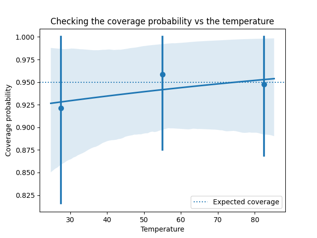
This looks reasonable - the calibration seems to be about 95%, regardless of the temperature.

What about a CI for a different GLM, like a logit model?

We’ve only spoken so far about the usual linear regression model, but we might wonder if we can compute CIs and PIs for Logit and other linear models, since they’re so closely related.

If we wanted to compute confidence intervals for models like a logit model, the procedure gets a bit more complicated due to the presence of the link function in the model. A common way of getting CIs for GLMs other than the usual OLS model is to use the delta method, which propagates the error for the parameters through the link function with a Taylor approximation. If you’re curious what that looks like for a logit model, I found this SE answer to be a useful example.

Luckily, with Statsmodels, we need not do this by hand either. While the Logit model in statsmodels doesn’t compute CIs, a GLMResults object returned from fitting a GLM with the binomial family has a get_prediction function just like the OLS example above.

Unlike a confidence interval, a prediction interval is a little less meaningful for a Logit model. For example, with a given $X$, we could compute the set of all the elements that we might plausibly see for $y$. However, for binary outcomes, the set is usually $\{0, 1\}$, because Logit models rarely assign zero probability to an event. As a result, this “prediction set” is usually not very useful.

Bonus: We can also simulate fake data points from our model

Here’s an interesting trick, which might be useful if you’d like to simulate some datasets we’d expect to see if the model were correct. Sometimes we want to do this when we impute missing data, or just because simulating data from a model tells us a lot about how the model does (or doesn’t) work. We can use the predicted mean for each datapoint, and sample from a normal distribution using that along with the SD of the prediction interval:

pr = results.get_prediction(df)
y_sim = np.random.normal(pr.predicted_mean, pr.se_obs)

For a Logit model, we could compute pr.predicted_mean in a similar way, then run it through np.random.binom(1, pr.predicted_mean) to get a simulated dataset of binary outcomes.

Appendix: Imports

from scipy.stats import norm
from matplotlib import pyplot as plt
import seaborn as sns
from statsmodels.api import formula as smf
import pandas as pd
import numpy as np

n = 100
a = 20
b = 9
s = 2

df = pd.DataFrame({'temperature': np.linspace(0, 110, n), 'sales':a + b*np.linspace(0, 1, n) + norm(0, s).rvs(n)})