Casual Inference Data analysis and other apocrypha
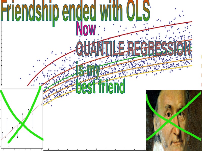
Understanding distributional impacts with Quantile Regression

p 8: http://www.econ.uiuc.edu/~roger/research/intro/rq3.pdf
from rdatasets import data
from statsmodels.api import formula as smf
from matplotlib import pyplot as plt
import seaborn as sns
import numpy as np

df = data('ISLR', 'Credit')

spec = 'Balance ~ Income + Limit + Rating + Cards + Education + Gender + Student + Married + Ethnicity'

ols_model = smf.ols(spec, df)
ols_fit = ols_model.fit()

Q = np.linspace(0.01, .99, 20)

quantreg_model = smf.quantreg(spec, df)
quantreg_fits = [quantreg_model.fit(q) for q in Q]

var_name = list(ols_fit.params.index)[-4] # Higher limit is associated with more spending; a higher limit shifts the whole distribution to the right, but lifts the left tail more than the right
alpha = 0.05

plt.ylabel(var_name)
plt.xlabel('Quantile')
plt.plot([Q[0], Q[-1]], [ols_fit.params[var_name], ols_fit.params[var_name]], color='red')
plt.fill_between([Q[0], Q[-1]],
         [ols_fit.conf_int(alpha)[0][var_name], ols_fit.conf_int(alpha)[0][var_name]],
         [ols_fit.conf_int(alpha)[1][var_name], ols_fit.conf_int(alpha)[1][var_name]],
         color='red', alpha=.1)
plt.plot(Q,
         [q_fit.params[var_name] for q_fit in quantreg_fits], color='blue')
plt.fill_between(Q,
                 [q_fit.conf_int(alpha)[0][var_name] for q_fit in quantreg_fits],
                 [q_fit.conf_int(alpha)[1][var_name] for q_fit in quantreg_fits],
                 alpha=.1,
                 color='blue')
plt.show()
Feel free to share!