Casual Inference Data analysis and other apocrypha
Conjugate priors for normal (and not-so-normal) data: The Normal-Gamma model in Python
If we take in our hand any volume; of divinity or school metaphysics, for instance; let us ask, Does it contain any abstract reasoning concerning quantity or number? No. Does it contain any experimental reasoning, concerning matter of fact and existence? No. Commit it then to the flames: for it can contain nothing but sophistry and illusion. An Enquiry Concerning Human Understanding (1748) sect. 12, pt. 3
Bayesian analysis of proportions using the beta conjugate prior is relatively easy to automate once you’ve got the basics down (this, this, and this are some good references if it’s a topic that’s new to you or you’d like a refresher). For practitioners using Python, it’s not much harder than from scipy.stats import beta. Analyzing the mean of continuous data is a little more slippery, though. The compound distribution named in the Wikipedia page, the frightening-sounding “Normal Gamma”, isn’t even implemented in scipy. What’s an analyst who just wants to evaluate a posterior distribution of the mean and variance to do?
Well, it turns out it’s not too bad - there’s just some assembly required. It’s worth a tour of the theory to get the context, and then we’ll do an example in Python.
A running example: Changes in clicks per customer
It’s often helpful to think about analysis techniques in terms of an example. We’ll take a look at an actual set of data to get a feel for how we might apply a normal conjugate prior in practice to understand the mean and variance of a distribution.
Let me set the scene. You’re the CBO (Chief Bayes Officer) of paweso.me, purveyor of deep learning blockchain AI targeted advertising for cats. You recently worked with some of your engineers to launch ChonkNet™, a Neural Network which predicts which users will buy which products (you’re hoping it’s an improvement on your current targeting model, DeepMeow™). You show a few thousand random users products based on the new algorithm, and measure the number of ads they clicks this week compared to compared to last week. The resulting per-user this week clicks - last week clicks looks like this:1
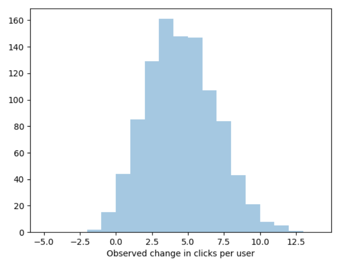
You’d like to know: What does the posterior of the mean and variance of revenue-per-user look like?
The usual story: Standard errors and confidence intervals
A quick refresher: In the classical story, quantities like “the population mean” and “the population variance” are actual properties of the population floating around in the world. We assume that the data we have were sampled from the population according to some random process, and then we make some inferences about what the population quantities might be. Usually, we can’t recover them exactly, but we can come up with a reasonable guess (a point estimate) and a range of variation based on the way the sampling happened (the confidence interval). If we like, we can even compute a statistic to gauge whether or not we can reject the hypothesis that our favorite population quantity is exactly zero, or test some other hypothesis we’re interested in (compute a P-value).
The kindest version of this story is one where the quantity we want is the population mean, the sampling is totally random, and we can appeal trust the Central Limit Theorem to tell us the sampling distribution of the mean. In that case, the sampling distribution of the mean is centered around the (unknown) true mean, and the standard deviation of the sampling distribution is the standard error.
The standard error of the mean is such an important formula that I’ll note it here. It will also turn out that the classical standard error has an important relationship with the Bayesian story we’re about to tell. If the mean of a random variable is $\mu$, the standard deviation is $\sigma$, and the sample size is $n$, then the standard error is
\[SE_\mu = \frac{\sigma}{\sqrt{n}}\]In practice, we often don’t know the population standard deviation, $\sigma$. When the sample is “large”, we’re usually willing to use $\hat{\sigma}$, a point estimate of sigma computed from the data. This sweeps a bit of uncertainty associated with sigma under the rug - if we wanted to avoid doing so, we’d use a slightly different procedure based on the T-distribution.
The standard error is so valuable in part because it lets us construct a confidence interval around the sample mean. The idea is that if we always constructed the CI at level $\alpha$ around the sample mean, our interval will contain the true mean most of the time. Specifically, we’d only leave it out $\alpha$ proportion of the time.
In the case of our datast from above, we might produce something like this:
from scipy.stats import norm

se = np.std(changes_in_clicks ) / np.sqrt(len(changes_in_clicks ))

print('The 99% confidence interval: {0}'.format(norm.interval(0.99, loc=np.mean(changes_in_clicks ), scale=se)))
Output:
The 99% confidence interval: (3.8489829444627057, 4.2390170555372935)
So the classical analysis would tell us that the week-over-week change in clicks per user is between about 3.84 and 4.24 at the 99% level.
A Refresher: Priors, Posteriors, Likelihoods, and Bayesian updates
The Bayesian perspective is a little different. Like the classical picture, it involves two parameters of interest - the mean and the variance, commonly referred to as $\mu$ and $\sigma^2$.. We’d like to learn something about these values of these parameters from the data. The Bayesian procedure involves a few steps:
- Write down your prior, $\mathbb{P}(\mu, \sigma)$, which summarizes all the information you have about $\mu$ and $\sigma$ before you see the data. This might be as vague as “every value of these parameters is equally likely” or as specific as “I’m almost entirely sure that $\mu$ is between 2 and 4”.
- Pick a Likelihood function $\mathcal{L}(X_1, …, X_n | \mu, \sigma)$ that relates the data to a potential value of the parameters.
- Look at the observed data, the values of $X$ that actually showed up in our dataset.
- Use Bayes Theorem to update the prior and get the posterior, $\mathbb{P}(\mu, \sigma | X_1, …, X_n)$.
We can look at the posterior to learn everything we want to know
The Bayesian version
In the both the Bayesian and classical version of this story, we’re interested in learning about the mean. In the last section, we compute a point estimate of the mean, and then come up with the standard error to construct confidence intervals around that estimate. From the Bayesian perspective, we choose a prior distribution, then combine it with the data to get a posterior distribution that tells us about our knowledge of the mean’s value.
The main difference between these views is that in the classical view, all our knowledge comes from the sampling distribution and what the data tells us about it. In the Bayesian view, all our knowledge comes from the posterior distribution we calculate from the prior and the data. Endnote: It’s not worth discusssing the philosophical differences between these two perspectives in detail right now. There are real advantages and disadvantages to the tools developed by both sides to be discussed another time, but the idea of a century-long holy war between Bayesians and Frequentists is overrated when we can all be pragmatists.
Let’s assume we know the variance (We often don’t know the true variance. a quick fix is to plug in the estimated variance and act as if that’s the real variance. if that makes you nervous, don’t worry - we’ll explore the implications of it a little later
Wiki says:
\[\mu | \mu_0, \sigma_0, \sigma, n \sim N(\mu_{post}, \sigma_{post})\] \[\mu_{post} = \frac{1}{\frac{1}{\sigma_0^2} + \frac{n}{\sigma^2}} \left ( \frac{\mu_0}{\sigma_0^2} + \frac{\sum_i x_i}{\sigma^2} \right )\] \[\sigma_{post}^2 = \left (\frac{1}{\sigma_0^2} + \frac{n}{\sigma^2} \right) ^{-1}\]woah now. let’s break that down - how does changing these parameters affect our inference
Digression: The posterior of the mean is closely connected to the standard error of the mean
You might start to wonder at this point whether or not all this Bayesian business offers a solution that contradicts the classical analysis. It turns out that they’re very closely related.
\[\lim_{\mu_0 \rightarrow 0, \sigma_0 \rightarrow \infty}\mu_{post} = \frac{1}{0 + \frac{n}{\sigma^2}} \left ( 0 + \frac{\sum_i x_i}{\sigma^2} \right ) =\frac{\frac{\sum_i x_i}{\sigma^2}}{\frac{n}{\sigma^2}} = \frac{\sum_i x_i}{n}\] \[\lim_{\mu_0 \rightarrow 0, \sigma_0 \rightarrow \infty} \sigma_{post}^2 = \left (\frac{1}{\sigma_0^2} + \frac{n}{\sigma^2} \right) ^{-1} = \frac{\sigma^2}{n} = SE_\mu^2\]How should I pick my prior?
We usually aren’t totally ignorant about the quantity of interest. For example, in the case of the change in clicks per user, we usually have seen this quantity in the past. Let’s say that in the past:
- The average change in clicks per user WoW is about zero. Maybe that’s different for holiday weeks or National Cat Day, but the week in question isn’t one of those.
- The average change in clicks per user WoW is “almost never” more than +10 or -10. (Perhaps those are the 1st and 99th percentiles of the empirical data we have).
This is exactly the kind of substantive information we often have access to in a realistic setting, even a very simple one. We’ll use these basic pieces of information to discuss a few possible choices of prior, based on some recommendations from the Stan docs. We’ll also look at how sensitive our inference is to the choice of prior, at least for this dataset.
A super-vague prior: N(0, 100000)
Often, when we talk about a “flat prior”, or and “uninformative prior” (both somewhat misleading terms), this is what we’re talking about. Sometimes, we justify this to ourselves by saying that it “lets the data speak for itself”, despite the fact that that phrase is always a vicious lie. As we noted in the last section, this prior will produce just about the same result as the classical analysis. Though you’ll get to tell your boss you used a “Bayesian method”, and maybe that’s worth something to you.
For the Bayes-skeptical, this is a choice that will let you feel like you’re on familiar ground. Those of you who have not yet accepted Reverend Thomas Bayes into your heart may .
A weak informed prior: N(0, 10)
This looks a little more informed, but it’s still quite permissive.
An actually informed prior: N(0, 3)
This actually reflects the facts above.
Lets compare all of these
import numpy as np
import seaborn as sns
from matplotlib import pyplot as plt
from scipy.stats import norm

def unknown_mean_conjugate_analysis(X, mu_0, sig_0):
  n = len(X)
  sd = np.std(X)
  m = np.mean(X)
  mu_post = ((mu_0/sig_0**2) + (m / sd**2)) / ((1/sig_0**2) + (n / sd**2))
  sig_2_post = 1. / ((1./sig_0**2) + (n / sd**2))
  return norm(mu_post, np.sqrt(sig_2_post))

posterior_super_vague = unknown_mean_conjugate_analysis(changes_in_clicks, 0, 100000)
posterior_weak = unknown_mean_conjugate_analysis(changes_in_clicks, 0, 10)
posterior_informed = unknown_mean_conjugate_analysis(changes_in_clicks, 0, 3)
But I don’t know the variance!! All this talk of $\hat{\sigma}$ is making me very nervous
Okay, okay! Let’s see how we might incorporate the uncertainty about the variance into our analysis, and how that changes our analysis if we mainly care about the mean - if the variance is a “nuisance parameter”, as it often is.
If we don’t: Normal Gamma
\[\mu, \tau \sim N \Gamma (\mu_0, \nu, \alpha, \beta)\]We observe $x$
| Parameter | Updated value | Flat prior value | Posterior value when prior is flat |
|---|---|---|---|
| $\mu_0$ | $\frac{\nu \mu_0 + n \bar{x}}{\nu + n}$ | $0$ | $\bar{x}$ |
| $\nu$ | $\nu + n$ | $0$ | $n$ |
| $\alpha$ | $\alpha + \frac{n}{2}$ | $-\frac{1}{2}$ | $\frac{n}{2} - \frac{1}{2}$ |
| $\beta$ | $$ |
Unlike in the known-variance case, this does not really produce
https://github.com/urigoren/conjugate_prior/blob/master/conjugate_prior/invgamma.py
from scipy.stats import gamma
import numpy as np
import seaborn as sns
from matplotlib import pyplot as plt

a = -0.5 # This recovers the bessel-corrected MLE; maybe that's an endnote though since it's not a real prior (but I won't tell if you won't)
b = 0

x = np.random.normal(0, 1, 10)
a_posterior = a + len(x) / 2
b_posterior = b + (0.5 * np.sum((x - np.mean(x))**2))
prec_posterior = gamma(a_posterior, scale=1./b_posterior)
precision_samples = prec_posterior.rvs(1000)
var_samples = 1./precision_samples
sns.distplot(var_samples)
plt.axvline(np.var(x, ddof=1))
plt.axvline(1./prec_posterior.mean(), color='orange', linestyle='dotted')
plt.show()
# An intuitive justification for the Gamma(0, 0) prior - Variance prior is arbitrarily broad
eps_choices = np.linspace(1e1, 1e-6, 500)
lower = np.array([gamma(eps, scale=1./eps).interval(.99)[0] for eps in eps_choices])
upper = np.array([gamma(eps, scale=1./eps).interval(.99)[1] for eps in eps_choices])
plt.plot(eps_choices, 1./lower, label='Upper')
plt.plot(eps_choices, 1./upper, label='Lower')
plt.xscale('log')
plt.yscale('log')
plt.legend()
plt.title('Upper and lower bounds on prior variance as epsilon changes')
plt.show()
Endnote stuff: (1) This isn’t a real prior so what is it (2) Bessel correction (3) This illustrates from the Bayesian point of view why the normal distribution isn’t a great posterior when the sample is small but the T-distribution is; the normal distribution doesn’t include the uncertainty from the unknown variance, leading to thinner tails.
https://stackoverflow.com/questions/42150965/how-to-plot-gamma-distribution-with-alpha-and-beta-parameters-in-python
https://en.wikipedia.org/wiki/Normal-gamma_distribution#Generating_normal-gamma_random_variates
How should I pick my prior? Variance edition
v = 0, mean = 0, alpha=0, beta=0
When we use the above prior it corresponds to MLE and has good frequentist properties
How essential is it that my data look normal
I mean what are a few outliers among friends eh
This shows up when the data are averages
Simulation of an almost-normal example
Large sample size usually makes up for non-normality; https://dspace.mit.edu/bitstream/handle/1721.1/45587/18-441Spring-2002/NR/rdonlyres/Mathematics/18-441Statistical-InferenceSpring2002/C4505E54-35C3-420B-B754-75D763B8A60D/0/feb192002.pdf
compare with Bayesian bootstrap
https://scholarsarchive.byu.edu/cgi/viewcontent.cgi?article=1277&context=facpub
An extra tip: What if my data is Log Normal instead of Normal?
Here’s a neat trick.
Endnotes
1 Okay, fine, that’s not real data; ChonkNet™ remains just an unrealized daydream in the head of one data scientist. I actually generated this data with this code:
from matplotlib import pyplot as plt
import seaborn as sns
import numpy as np
from scipy.stats import skellam

np.random.seed(7312020)

changes_in_clicks = skellam(40, 20).rvs(1000)

sns.distplot(changes_in_clicks, kde=False)
plt.xlabel('Observed change in clicks per user')
plt.show()
The idea is that the number of clicks is Poisson distributed in each week, and the Skellam distribution is the distribution of the difference between two Poisson distributions. So this is hopefully a plausible set of data that we might see from the difference of two weekly click datasets.
Written on th, by Louis Cialdella