Would collecting more data improve my model's predictions? The learning curve and the value of incremental samples

Since we usually need to pay for data (either with money to buy it or effort to collect it), it’s worth knowing the value of getting more data points to fit your predictive model. We’ll explore the learning curve, a model-agnostic way of understanding how performance changes as we add more data points to our sample. Analysis of the learning curve tells us whether it’s worth it to collect a larger dataset, and it’s easy to do this analysis in Python with scikit-learn.

Is it worth collecting more samples?

When we have a sample of data we want to use to fit a model, it’s natural to ask ourselves whether we have “enough” samples on hand. Would collecting more data improve our model, or has it reached a performance plateau? This is a question with a lot of practical importance, because data is expensive! We need to pay to acquire samples - either literally exchanging money with a data vendor or building systems to collect data. When our analysis is simple, like a difference in means, we can achieve this by computing the power of a hypothesis test or the precision of the effect size confidence interval. But if you have a carefully-crafted regression model or black-box machine learning model, it’s a lot less clear how to gauge whether you have enough samples.

For example, let’s say you’ve already collected a number of datapoints about Portugese wine using a combination of chemical analysis and human rating of some sample wines. You’d like to build a predictive model that relates the measurable chemical properties of wine to its quality, perhaps so you can sell it to a Portugese Winery to automate their quality assurance. You’ve just done some fancy model selection and decided that a Lasso model will probably give you the best trade-off between prediction quality and model simplicity. You’ve already went through some effort to gather the 1,599 samples of wine measurements in your data set; but perhaps your model would make better predictions if you collected even more samples? On the one hand, this would probably be expensive. You’ll have to have some more wine analyzed, and get human raters to tell you more about their preferences. On the other hand, this investment might make your model more valuable (wineries might be willing to pay more to secure certain production standards), making the acquisition of the data worth it.

In order to answer this question, let’s think about what information would be sufficient to answer it. The simplest thing that comes to my mind is the relationship between the sample size and the quality of the model - if we knew that, we could figure out if it’s likely that more data would provide incremental value to your model’s predictive ability.

The learning curve tells us how model performance varies with sample size

The relationship between sample size and model quality has a name: the learning curve. The learning curve is a plot of how the model’s performance on our favorite metric (like MSE or ROC-AUC varies with sample size). Sometimes we’ll plot both the in-sample (training) and out-of-sample (validation) performance together; we’ll just focus on the out-of-sample performance for now.

We have some intuition about the shape of this curve. As the number of samples grows, the performance of the model usually improves rapidly and then “flattens out” until adding more data points has little effect. We’ll make the assumption that this family of shape describes the curve, and the main question is whether we’re currently in the steeply rising part of the curve, or the flatter part. This doesn’t strike me as a very strong assumption, since I haven’t seen any examples of real-life models where the model performance “jumps” after being flat for a large number of samples. Nonetheless, this is an assumption, and we should be careful to take note of it.

Let’s plot the learning curve for the RMSE of our Lasso model on our Portugese wine data set. As usual, we can have our old friend scikit-learn do all the hard work. This piece of code is adapted from their learning curve example. The library will run K-fold CV at varying sample sizes, giving us a mean and variance around the RMSE as the sample size changes. We’ll use 10-fold splitting.

You can find the imports and code to fetch the data in the appendix.

n_folds = 10

train_sizes, _, test_scores = learning_curve(Lasso(alpha=10**(-3), normalize=True), X, y, cv=n_folds, scoring='neg_root_mean_squared_error', train_sizes=np.linspace(0.1, 1, 20))
test_scores = -test_scores
test_scores_mean = np.mean(test_scores, axis=1)
test_scores_se = np.std(test_scores, axis=1) / np.sqrt(n_folds)
test_scores_var = test_scores_se**2

We can then plot the relationship between sample size and model performance:

plt.plot(train_sizes, test_scores_mean, marker='o', label='Mean')
plt.fill_between(train_sizes, test_scores_mean - 1.96 * test_scores_se, test_scores_mean + 1.96 * test_scores_se, alpha=.1, label='CI')
plt.title('Learning Curve for Lasso model')
plt.xlabel('Sample size')
plt.ylabel('CV RMSE')
plt.tight_layout()
plt.legend()
plt.show()

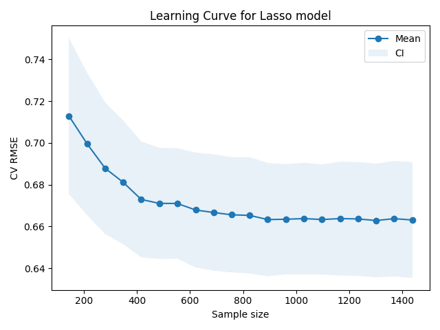
So far, so good. This learning curve has exactly the kind of shape we’d expect. The error drops steeply as we add the few batches of samples, but seems to “saturate” after a few hundred samples, as adding more data makes little impact. However, it can be a little tough to tell what’s going on with the right hand side of the graph. It looks like the incremental data points there are providing relatively little value, but it’s worth taking a closer look.

The incremental value of a data point

The question here is whether adding a new batch of samples from the same source (a presumed IID one) would provide value by decreasing the model’s RMSE. Our learning curve tells us about the performance of the model at each sample size, and we can transform it to learn about the incremental value of each batch of samples. We’ll take the first difference of the learning curve using np.diff. This will tell us the incremental value we observed for each batch of data points we added to the model; specifically, we’ll get the change in the RMSE when that batch was added.

mean_diff = np.diff(test_scores_mean)
diff_se = np.sqrt(test_scores_var[1:] + test_scores_var[:-1])

diff_df = pd.DataFrame({'mean_diff': mean_diff, 
                        'n': train_sizes[1:]})

spline_fit = smf.wls('mean_diff ~ bs(n, df=3)', diff_df, weights=1./diff_se**2).fit() # Differing variances of observations

y_pred_df = spline_fit.get_prediction(diff_df).summary_frame(alpha=.05)

plt.scatter(diff_df['n'], diff_df['mean_diff'], label='Observed CV error')
plt.plot(diff_df['n'], y_pred_df['mean'], label='Smoothed error')
plt.fill_between(diff_df['n'], y_pred_df['mean_ci_lower'], y_pred_df['mean_ci_upper'], alpha=.1, color='blue', label='CI')
plt.axhline(0, linestyle='dotted')
plt.xlabel('Sample size')
plt.ylabel('Improvement in RMSE')
plt.title('First difference of learning curve')
plt.tight_layout()
plt.legend()
plt.show()

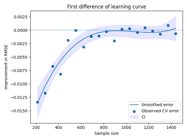
We see that the first 800 data points are by far the most valuable. Each incremental data point from 0 to 800 seems to have meaningfully reduced the RMSE. However, after around a sample size of 800, the incremental data points seem to provide relatively little value. In order to make the “path” here clear, I also plotted a smoothed version using a cubic B-Spline with 3 knots. You could achieve a similar result using your favorite smoother, like a moving average or lowess.

And with this, we have an answer to our initial question. Collecting more data by sending more wine to the laboratory is likely to be a poor investment with the model we’ve chosen. It looks like we could have done reasonably well with about 1000 data points, even; not much improvement seems to occur after that.

I should point out here that in general, there’s no “rule of thumb” for what the learning curve looks like or when it flattens out. You’ll need more data when the model is more complex, or your features are highly correlated, or when you have a lot of classes you’re predicting. This method lets you assess the value of a given simple size for whatever crazy black-box model you’ve dreamed up, without having to do much ad hoc setup.

Putting it all together: Computing the value of a larger sample

That was a lot! Let’s recap it quickly, to make it clear what the process is by which we answer our original question.

• You have a sample on hand, and a particular model you’ve decided to fit to it so you can make predictions. You’d like to know if collecting more samples would improve your model’s predictive power.
• Compute the learning curve for your favorite model, to get a feel for how the sample sizes affects the model’s quality. Does the learning curve flatten out out as we approach the current sample size, or does it still have a large slope?
• Calculate the first difference of the learning curve, and see if that first difference is about zero near the current sample size. Consider smoothing this curve to see if it has a mean of zero on the farthest part of the curve. If the first difference has “settled down” around zero, adding more samples likely won’t improve things.

Appendix: Setup and imports

We download the data:

curl http://www3.dsi.uminho.pt/pcortez/wine/winequality.zip --output winequality.zip
unzip winequality.zip
cd winequality/

Plus import libraries and read from the CSV:

from sklearn.linear_model import Lasso
from sklearn.model_selection import learning_curve
import numpy as np
from matplotlib import pyplot as plt
import seaborn as sns
import pandas as pd
from statsmodels.api import formula as smf
from sklearn.utils import resample

df = pd.read_csv('winequality-red.csv', sep=';')

y = df['quality']
X = df.drop('quality', axis=1)